Other Topics

2.8 Other Topics

The following section serves as a repository for mathematical derivations and identities which are used later in this book.

2.8.1 Trigonometric Approximations

Consider the Taylor series approximation for $\sin (x)$ centered at $x = 0$ , provided in table 2.4 and rewritten in equation 2.292 for continuity.

\sin (x) = x - \frac{x^{3}}{3!} + \frac{x^{5}}{5!} - \frac{x^{7}}{7!} + . . . + {(- 1)}^{n} \frac{x^{2 n + 1}}{(2 n + 1)!}

(2.292)

We can rewrite equation 2.292 as shown in equations 2.293 and 2.294.

\sin (x) = x + e r_{t}

(2.293)

e r_{t} = - \frac{x^{3}}{3!} + \frac{x^{5}}{5!} - \frac{x^{7}}{7!} + . . . + {(- 1)}^{n} \frac{x^{2 n + 1}}{(2 n + 1)!}

(2.294)

In equations 2.293 and 2.294, $e r_{t}$ stands for error truncation terms. For relatively small values $x$ , $e r_{t}$ will be small. This is shown in Table 2.5, where values of $\sin (x)$ and $e r_{t}$ are compared for given values of $x$ . Therefore, we can simply replace $\sin (x)$ in a given equation with $x$ since $\sin (x) \approx x$ at small $x$ values which have low $e r_{t}$ . This is referred to as the small angle approximation.

Table 2.5: Table showing

x

values,

\sin x

values, and the difference

e r_{t} = x - \sin x

$x$	$e r_{t}$	$\sin (x)$

0	0	0
0.1	0.00016	0.09983
0.5	0.02057	0.47942
1	0.15852	0.84147

A similar method can be used to show that for small values of $x$ the small angle approximation $\tan (x) \approx x$ .

2.8.2 Coordinate axis rotation

In this book, many problems will utilize a coordinate axis or reference frame. At times, this reference frame needs to be rotated. In this section, we will derive the new coordinates of a particle $x_{r}, y_{r}$ after rotating it’s frame of reference by distance $𝜃$ from the original coordinate system $x, y$ . In doing this, please consider the Figure 2.14.

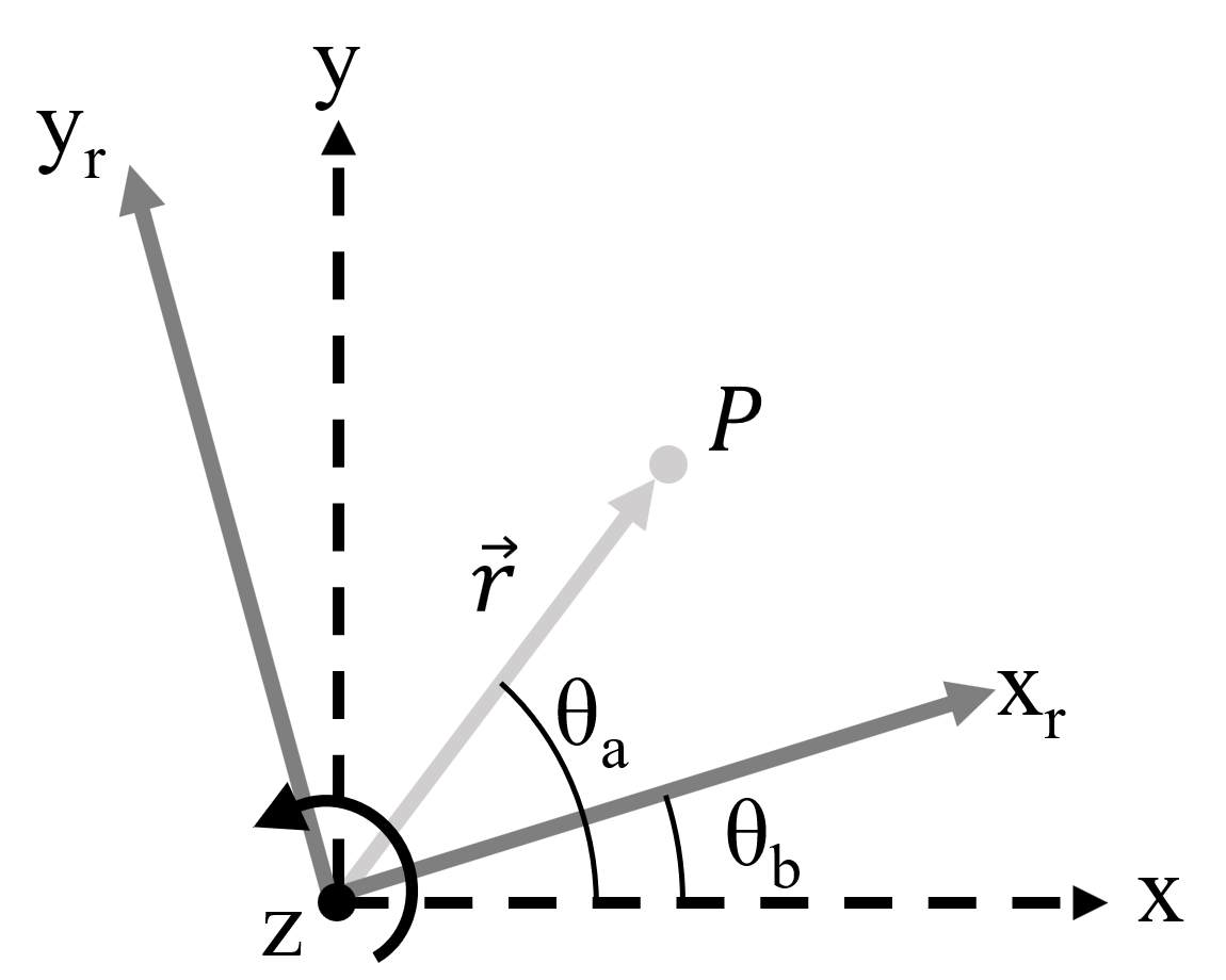
Figure 2.14: Coordinate axis rotation from $x, y$ to $x_{r}, y_{r}$

Let us analyze point $P$ indicated by distance from the origin $\vec{r}$ and angle $𝜃_{a}$ . By definition we know the following is true for the coordinates of $P$ in the $x, y$ coordinate system:

\begin{align} x = | r | \cos (𝜃_{a}) & (2.295) \\ y = | r | \sin (𝜃_{a}) & (2.296) \end{align}

We also know the following is true for the coordinates of $P$ in the $x_{r}, y_{r}$ coordinate system:

\begin{array}{l} x_{r} = | r | \cos (𝜃_{a} - 𝜃_{b}) \end{array}

\begin{array}{l} y_{r} = | r | \sin (𝜃_{a} - 𝜃_{b}) \end{array}

From trigonometry we can get the following identities:

\begin{align} | r | \cos (𝜃_{a} - 𝜃_{b}) = | r | \cos (𝜃_{a}) \cos (𝜃_{b}) + | r | \sin (𝜃_{a}) \sin (𝜃_{b}) & (2.297) \end{align}

\begin{align} | r | \sin (𝜃_{a} - 𝜃_{b}) = | r | \sin (𝜃_{a}) \cos (𝜃_{b}) - | r | \cos (𝜃_{a}) \sin (𝜃_{b}) & (2.298) \end{align}

Plugging 2.295 and 2.296 into 2.297 and 2.298, we get the following:

\begin{align} x_{r} = x * \cos (𝜃_{b}) + y * \sin (𝜃_{b}) & (2.299) \\ y_{r} = - x * \sin (𝜃_{b}) + y * \cos (𝜃_{b}) & (2.300) \end{align}

We can rewrite equations 2.299 and 2.300 in matrix form as shown in equation 2.301.

[\begin{matrix} x_{r} \\ y_{r} \end{matrix}] = [\begin{matrix} \cos (𝜃_{b}) & \sin (𝜃_{b}) \\ - \sin (𝜃_{b}) & \cos (𝜃_{b}) \end{matrix}] [\begin{matrix} x \\ y \end{matrix}]

(2.301)

To go from $(x_{r}, y_{r})$ to $(x, y)$ , we simply take the inverse of the matrix (section 2.6.0.0) to get equation 2.302.

[\begin{matrix} x \\ y \end{matrix}] = [\begin{matrix} \cos (𝜃_{b}) & - \sin (𝜃_{b}) \\ \sin (𝜃_{b}) & \cos (𝜃_{b}) \end{matrix}] [\begin{matrix} x_{r} \\ y_{r} \end{matrix}]

(2.302)

For a three dimensional coordinate axis rotation, we must consider there are three possible ways the coordinate axis can be rotated; about the x-axis ( $𝜃_{x}$ ), about the y-axis ( $𝜃_{y}$ ), and about the z-axis ( $𝜃_{z}$ ). Each of these rotations has a matrix associated with it, dubbed the ”rotation matrix”. The x-axis rotation matrix is provided in equation 2.303.

R_{x} (𝜃_{x}) = [\begin{matrix} 1 & 0 & 0 \\ 0 & \cos (𝜃_{x}) & - \sin (𝜃_{x}) \\ 0 & \sin (𝜃_{x}) & \cos (𝜃_{x}) \end{matrix}]

(2.303)

The y-axis rotation matrix is provided in equation 2.304.

R_{y} (𝜃_{y}) = [\begin{matrix} \cos (𝜃_{y}) & 0 & \sin (𝜃_{y}) \\ 0 & 1 & 0 \\ - \sin (𝜃_{y}) & 0 & \cos (𝜃_{y}) \end{matrix}]

(2.304)

The z-axis rotation matrix is provided in equation 2.305.

R_{z} (𝜃_{z}) = [\begin{matrix} \cos (𝜃_{z}) & - \sin (𝜃_{z}) & 0 \\ \sin (𝜃_{z}) & \cos (𝜃_{z}) & 0 \\ 0 & 0 & 1 \end{matrix}]

(2.305)

In addition, the order in which we rotate matters; if we rotate our coordinate system about the x-axis, the y-axis will move. Therefore, if our next rotation is about the ”new” y-axis, a different rotation will be achieved than if we rotate about the original y-axis. In addition, it matters about what coordinate system we rotate. In an extrinsic rotation, each subsequent rotation occurs about a fixed coordinate system. In an intrinsic, each subsequent rotation occurs about the new coordinate system that results from the previous rotation. An extrinsic rotation that occurs about fixed axes $x$ , then $y$ , then $z$ can be conducted using equation 2.306.

[\begin{matrix} x \\ y \\ z \end{matrix}] = R_{z} (𝜃_{z}) R_{y} (𝜃_{y}) R_{x} (𝜃_{x}) [\begin{matrix} x_{r} \\ y_{r} \\ z_{r} \end{matrix}]

(2.306)

An intrinsic rotation about axes $x$ , then the new $y$ , and then the new $z$ can be conducted using equation 2.307.

[\begin{matrix} x \\ y \\ z \end{matrix}] = R_{x} (𝜃_{x}) R_{y} (𝜃_{y}) R_{z} (𝜃_{z}) [\begin{matrix} x_{r} \\ y_{r} \\ z_{r} \end{matrix}]

(2.307)

As shown in equation 2.307, an intrinsic rotation has the reverse order of the extrinsic rotation.

2.8.3 Imaginary Numbers

The imaginary number, symbolized by $i$ , is a term that is used to define the square root of -1 as shown in equation 2.308.

\begin{align} i = \sqrt{- 1} & (2.308) \end{align}

There is nothing imaginary about the imaginary number. In fact, the use of the word “imaginary” makes the imaginary number seem far more mysterious than it is. In the following paragraphs it will be shown that applying the same mathematical rules to imaginary numbers that we use for real numbers leads to very useful and interesting results.

Numbers that combine real and imaginary numbers are called complex numbers. There are two forms in which complex numbers can be expressed; these are the polar form and Cartesian form (sometimes called rectangular form). A generalized complex number in the polar form is shown in equation 2.309.

\begin{align} z = r e^{𝑖𝜃} & (2.309) \end{align}

In equation 2.309, $r$ is called the magnitude of the complex number and is also expressed as $| z |$ . A generalized complex number written in Cartesian form is shown in equation 2.310.

\begin{align} z = x \pm 𝑦𝑖 & (2.310) \end{align}

Polar form can be converted to Cartesian form by use of Euler’s identity (equation 2.248) as shown in equation 2.311.

\begin{matrix} \begin{aligned} x = r \cos (𝜃) \\ y = r \sin (𝜃) \end{aligned} \end{matrix}

(2.311)

The complex conjugate of a given complex number provided in Cartesian form is defined as a number which has the same real part as the original number, but an opposite imaginary part. To find the magnitude of a complex number provided in Cartesian form, we take the square root of the product of the number multiplied by it’s complex conjugate as shown in equation 2.312.

\begin{align} r = | z | = \sqrt{(x + 𝑦𝑖) (x - 𝑦𝑖)} = \sqrt{x^{2} + y^{2}} & (2.312) \end{align}

To add two complex numbers $z_{1}$ and $z_{2}$ we simply individually add the real and imaginary components. To do this, we use the Cartesian form as shown in equation 2.313.

\begin{align} z_{1} + z_{2} = x_{1} + x_{2} + (y_{1} + y_{2}) i & (2.313) \end{align}

Similarly, to subtract two complex numbers $z_{2}$ from $z_{1}$ we subtract the real and imaginary parts individually. As with addition, to do this we use Cartesian form as shown in equation 2.314.

\begin{align} z_{1} - z_{2} = x_{1} - x_{2} + (y_{1} - y_{2}) i & (2.314) \end{align}

To multiply complex numbers in polar form, we can use rules of exponents and simply add the exponents as shown in equation 2.315.

\begin{align} z_{1} z_{2} = r_{1} r_{2} e^{i (𝜃_{1} + 𝜃_{2})} & (2.315) \end{align}

To multiply complex numbers in Cartesian form, we can foil as shown in equation 2.316.

\begin{align} z_{1} z_{2} = (x_{1} x_{2} - y_{1} y_{2}) + (x_{1} y_{2} + x_{2} y_{1}) i & (2.316) \end{align}

To divide complex numbers in polar form, we can again use the rules of exponents as shown in equation 2.317.

\begin{align} \frac{z_{1}}{z_{2}} = \frac{r_{1}}{r_{2}} e^{i (𝜃_{1} - 𝜃_{2})} & (2.317) \end{align}

To divide complex numbers in Cartesian form, we must first multiply the denominator (the term we are dividing by) by it’s complex conjugate as shown in equation 2.318.

\begin{align} \frac{z_{1}}{z_{2}} = \frac{x_{1} + y_{1} i}{x_{2} + y_{2} i} * \frac{x_{2} + y_{2} i}{x_{2} - y_{2} i} & (2.318) \end{align}

Simplifying equation 2.319, you may notice that the denominator becomes $| z_{2} |^{2}$ which is a real number. Therefore, our simplified quotient is shown in equation 2.319

\begin{align} \frac{z_{1}}{z_{2}} = \frac{x_{1} x_{2} - y_{1} y_{2}}{| z_{2} |^{2}} + \frac{x_{1} y_{2} + x_{2} y_{1}}{| z_{2} |^{2}} i & (2.319) \end{align}

Complex functions

A complex function is a function which acts on a complex number. This means that a complex number is taken in by the function and based on this input, a complex number is output by the function. Therefore, if our input is $x + 𝑦𝑖$ then our output will be $u (x, y) + v (x, y) i$ as shown in equation 2.320.

\begin{align} f (z) = f (x + 𝑦𝑖) = u (x, y) + v (x, y) i & (2.320) \end{align}

In equation 2.320, $u$ is a real valued function of $(x, y)$ which constitutes the real part of the function output, and $v$ is another real valued function of $(x, y)$ which constitutes the imaginary part of the function output.

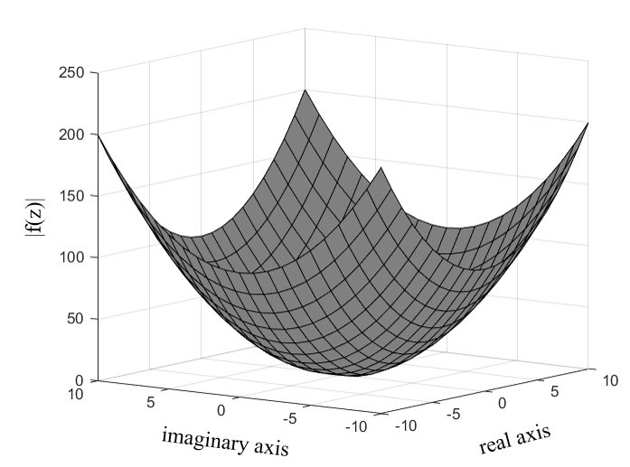
An example of a complex function is provided in equation 2.321.

\begin{align} f (z) = z^{2} + 1 & (2.321) \end{align}

Plugging in the Cartesian form of a complex number (equation 2.310)for $z$ , we get equation 2.322.

\begin{align} f (z) = (x^{2} - y^{2} + 1) + (2 𝑥𝑦) i & (2.322) \end{align}

From equation 2.322, we can clearly see that $u (x, y) = x^{2} - y^{2} + 1$ , and $v (x, y) = 2 𝑥𝑦$ . A fundamental constraint with the graphing a complex functions is that we have two inputs $x$ and $y$ along with two outputs $u (x, y)$ and $v (x, y)$ , making this a four dimensional dataset which cannot be easily shown in three dimensions. Therefore, the magnitude $| f (z) |$ is typically plotted as a function of $x$ and $y$ . Such a plot is for the function in equation 2.322 is shown in Figure 2.15.

Figure 2.15: $| f (z) |$ as a function of $x$ and $y$ for equation 2.322.

Why complex numbers are commonly used to model waves

Waves are fundamentally sinusoidal functions (either $\sin (𝜃)$ or $\cos (𝜃)$ ). In many physics/engineering applications, we are interested in adding, subtracting, multiplying, and dividing wave functions (i.e. sinusoidal functions). From Euler’s identity (equation 2.248), we know that a complex number is sinusoidal in nature making it eligible for modeling waves. In addition, operating on complex numbers is relatively simple due to the availability of both the Cartesian and polar forms; adding/subtracting (equations 2.313 and 2.314) is easily done in Cartesian form, while multiplying/dividing (equations 2.315 and 2.317) is easily done in polar form. This simplicity of operations is why complex numbers are commonly used to model waves.