Differential Equations

2.2 Differential Equations

A differential equation is an equation that shows a relationship among derivatives. These derivatives may be multiplied by each other. They may also bare some relationship to the original function. There are many different types of differential equations. We will begin this section by reviewing differential equation classification.

Order

The order of a differential equation is the highest derivative within the differential equation. As an example, please consider equation 2.55.

y = \frac{d^{2} y}{d x^{2}} + \frac{𝑑𝑦}{𝑑𝑥}

(2.55)

The highest derivative in equation is $\frac{d^{2} y}{d x^{2}}$ . Therefore, this is a second order differential equation.

Partial vs. Ordinary

An ordinary differential equation is one composed of the derivatives of single variable functions. This type of derivative is introduced in section 2.1.1. Equation 2.56 shows an example of an ordinary differential equation.

y = \frac{d^{2} y}{d x^{2}} + \frac{𝑑𝑦}{𝑑𝑥}

(2.56)

A partial differential equation is, as the name suggests, composed of partial derivatives. As a reminder from section 2.1.2, this means that we are dealing with derivatives of a multi-variable function. Equation 2.57 shows an example of a partial differential equation.

0 = \frac{∂𝑧}{∂𝑥} + \frac{∂𝑧}{∂𝑦}

(2.57)

Linear vs. Non-Linear

A linear differential equation is a special type of ordinary differential equation that follows the following form shown in equation 2.58.

a_{n} (x) \frac{d^{n} y}{d x^{n}} + a_{n - 1} (x) \frac{d^{n - 1} y}{d x^{n - 1}} + . . . + a_{1} (x) \frac{𝑑𝑦}{𝑑𝑥} + a_{0} (x) y = g (x)

(2.58)

In equation 2.58, $y = f (x)$ . The important thing to note in equation 2.58 is that all values $y$ and all derivatives of $y$ are to the first power. In addition, no derivatives of $y$ are multiplied by $y$ . Therefore, this equation is said to be linear in $y$ . Please note that equation 2.58 accounts for the fact that the $a$ coefficients could be 0, therefore eliminating the derivative of that order from the equation. So an equation that does not have a $\frac{d^{2} y}{d x^{2}}$ term but has a $\frac{d^{3} y}{d x^{3}}$ and $\frac{𝑑𝑦}{𝑑𝑥}$ is still considered linear. Equation 2.59 shows an example of a linear differential equation.

\cos (x) \frac{𝑑𝑦}{𝑑𝑥} + x^{2} y = \cos^{2} (x) + \sin (2 x)

(2.59)

Equation 2.59 is linear in $y$ .

A non linear differential equation is one that does not follow the listed rules. Equation 2.60 shows example of a non-linear differential equation.

\cos (x) {(\frac{𝑑𝑦}{𝑑𝑥})}^{2} + x^{2} \sqrt{y} = \cos^{2} (x) + \sin (2 x)

(2.60)

Second+ Order Homogeneous vs. Non-Homogeneous

There are two definitions of a homogeneous differential equation. The first definition applies to first order differential equations. We will not cover this definition, because it is very specific. The second definition of homogeneous differential equations applies to second+ order differential equations. A differential equation with the desired solution $y = f (x)$ is said to be homogeneous if it follows the form shown in equation 2.61.

a_{n} (x) b_{n} (y) \frac{d^{n} y}{d x^{n}} + a_{n - 1} (x) b_{n - 1} (y) \frac{d^{n - 1} y}{d x^{n - 1}} + . . . + a_{1} (x) b_{1} (y) \frac{𝑑𝑦}{𝑑𝑥} + a_{0} (x) b_{0} (y) = 0

(2.61)

This is a similar equation as shown for linear differential equations. However, the important thing with homogeneous differential equations is that there is no $g (x)$ ; there are no standalone functions of the dependent variable (which, in the $y = f (x)$ functionality, is $x$ ).

An example of a homogeneous second order differential equation is shown in equation 2.62.

x \frac{d^{2} y}{d x^{2}} + y^{2} = 0

(2.62)

An example of a non-homogeneous second order differential equation is shown in equation 2.63.

x \frac{d^{2} y}{d x^{2}} + y^{2} = \sin (x)

(2.63)

Solving Differential Equations

As defined previously, a differential equation is simply a relationship of derivatives. Our goal is to decode this differential equation and find a function that satisfies it. In other words, if we are dealing with an ordinary differential equation, we want to find a function $y = f (x)$ that, if plugged into the differential equation, holds true. If working with a partial differential equation, we want to find a function $z = f (x, y, . . .)$ that, if plugged into the differential equation, holds true. I say “a” equation because theoretically, there could be multiple equations that serve as a solution to the differential equation. In the sections below we will go over methods for finding solutions to differential equations.

From section 2.1.1, we know that the derivative of a constant function is 0 (if the function is constant, its change must be $0$ ). This, in effect, leads to a situation that each time we take a derivative of a function we loose information regarding any constant terms within the function. Let us take a step back; we are looking for functions which comply with a set of derivative relationships. There are infinite constant terms that can be added to any function and still comply with the derivative relationship defined in the differential equation. For example, $5 x + 6$ has the same derivative as $5 x + 7$ . Typically, we lock these constant terms by including initial conditions or boundary conditions. Initial conditions, as the name suggests, specify the value of the function $f$ or its derivatives when the independent variable is $0$ . Boundary conditions specify the value of the function $f$ at given “boundary” values of the differential equation. The difference between initial conditions and boundary conditions can be nebulous when a boundary condition at $0$ is specified. Therefore, the naming of these conditions can be thought of as a technicality and not a critical aspect to solving differential equations. When we have an $𝑛𝑡h$ order differential equation, this means we must differentiate our solution-function $n$ times. Again, every time we differentiate we loose a constant term. Therefore, we need to have $n$ initial conditions/boundary conditions for a differential equation of order $n$ .

2.2.1 Direct Integration

Direct integration is a technique which can be used for first order ordinary differential equations which can be manipulated to the form shown in equation 2.64. Again, our goal is to find a equation $y = f (x)$ that satisfies the given differential equation.

N (y) \frac{𝑑𝑦}{𝑑𝑥} = M (x)

(2.64)

$N (y)$ is some function of $y$ and $M (x)$ is some function of $x$ . In this case, we can just directly integrate equation 2.64 with respect to $x$ . Doing this, we get equation 2.65.

\int N (y) \frac{𝑑𝑦}{𝑑𝑥} 𝑑𝑥 = \int M (x) 𝑑𝑥

(2.65)

The integral in equation 2.65 can be integrated using methods specified in section 2.1.5. Since this is a first order differential equation, we only need one initial condition to fully define its solution.

Short Example

Let us begin with the differential equation provided in equation 2.66.

2 y \frac{𝑑𝑦}{𝑑𝑥} = 3 x^{2} + 4 x - 4

(2.66)

We will find a solution to equation 2.66 given the initial conditions provided in equation 2.67.

f (0) = 1

(2.67)

Using the method outlined in equation 2.65, we get the equation 2.68.

\int 2 y \frac{𝑑𝑦}{𝑑𝑥} 𝑑𝑥 = \int 3 x^{2} + 4 x - 4 𝑑𝑥

(2.68)

Integrating equation 2.68, we get equation 2.69.

y^{2} + c_{1} = x^{3} + 2 x^{2} - 4 x + c_{2}

(2.69)

Both integrals generate a constant of integration. However, we could say that $C = c_{2} - c_{1}$ . In this case, we are left with equation 2.70.

y = \sqrt{x^{3} + 2 x^{2} - 4 x + C}

(2.70)

Equation 2.70 shows the general solution. It holds true for any constant $C$ . In order to specify this constant $C$ , we plug in the initial conditions specified in equation 2.67. Doing this, we get $C = 1$ . Therefore, our final solution is as shown in equation 2.71.

y = \sqrt{x^{3} + 2 x^{2} - 4 x + 1}

(2.71)

2.2.2 Substitution

The substitution method can be used to solve linear (in the dependent variable, which in this book is $y$ ) homogeneous differential equations, with the stipulation that there may be no independent ( $x$ ) variables within the equation. Therefore, these equations must be of the form shown in equation 2.72.

c_{n} \frac{d^{n} y}{d x^{n}} + c_{n - 1} \frac{d^{n - 1} y}{d x^{n - 1}} + . . . + c_{1} \frac{𝑑𝑦}{𝑑𝑥} + c_{0} (y) = 0

(2.72)

In equation 2.72, $c_{n}$ is a known constant. To solve equation 2.72 using the substitution method, we start with the assumption shown in equation 2.73.

y = e^{𝜆𝑥}

(2.73)

Assuming this, we can find the nth derivative of the above function using the chain rule (section 2.1.1.0) as shown in equation 2.74.

\frac{d^{n} y}{d x^{n}} = λ^{n} e^{𝜆𝑥}

(2.74)

Plugging equations generated using equation 2.74 into equation 2.72 we get equation 2.75.

c_{n} λ^{n} e^{𝜆𝑥} + c_{n - 1} λ^{n - 1} e^{𝜆𝑥} + . . . + c_{1} λ^{1} e^{𝜆𝑥} + c_{0} e^{𝜆𝑥} = 0

(2.75)

Factoring out $e^{𝜆𝑥}$ , we get equation 2.76.

e^{𝜆𝑥} (c_{n} λ^{n} + c_{n - 1} λ^{n - 1} + . . . + c_{1} λ^{1} + c_{0}) = 0

(2.76)

By the zero product property, we can separate the terms in equation 2.76 generating equations 2.77 and 2.78.

e^{𝜆𝑥} = 0

(2.77)

c_{n} λ^{n} + c_{n - 1} λ^{n - 1} + . . . + c_{1} λ^{1} + c_{0} = 0

(2.78)

Now, we know that $e^{𝜆𝑥}$ can never equal $0$ . Therefore, we are left with equation 2.78. You may notice that this equation is simply a polynomial which we can solve for $λ$ . We should get $n$ “roots”, which are values for lambda. In order to find the solution to our differential equation, we plug all of these $λ$ values back into equation 2.73. We then add all of these equations together. This is shown in equation 2.79.

y = C_{1} e^{λ_{1} x} + C_{2} e^{λ_{2} x} + . . . + C_{n} e^{λ_{n} x}

(2.79)

Equation 2.79 is the general solution; it has constants $C_{n}$ . As expected, the number of constants matches the order of the differential equation. In order to find the value of these constants, we use the initial conditions.

Short Example

Let us start with the differential equation listed in equation 2.80.

\frac{d^{2} y}{d x^{2}} - 4 \frac{𝑑𝑦}{𝑑𝑥} - 12 y = 0

(2.80)

The initial conditions are provided in equation 2.81.

\begin{matrix} \begin{aligned} f (0) & = 1 \\ \frac{𝑑𝑓 (0)}{𝑑𝑥} & = 0 \end{aligned} \end{matrix}

(2.81)

Following the prescribed methodology and arriving at the equation laid out by equation 2.78, we get equation 2.82.

λ^{2} - 4 λ - 12 = 0

(2.82)

Solving the polynomial in equation 2.82, we get values for lambda as shown in equations 2.83.

λ = - 2, 6

(2.83)

Therefore, per equation 2.79, our solution is shown in equation 2.84.

y = C_{1} e^{- 2 x} + C_{2} e^{6 x}

(2.84)

Using the initial conditions laid out in the problem statement (equation 2.81), we get $C_{1} = 3 ∕ 4$ and $C_{2} = 1 ∕ 4$ . Therefore, our final solution is shown in equation 2.85.

y = \frac{3}{4} e^{- 2 x} + \frac{1}{4} e^{6 x}

(2.85)

2.2.3 The Method of Undetermined Coefficients

The method of undetermined coefficients can be used to solve linear (in $y$ ) non-homogeneous differential equations with the stipulation that no functions of the independent variable ( $x$ ) may be multiplied by the dependent variable ( $y$ ) or its derivatives. Therefore, these equations must be of the form shown in equation 2.86.

c_{n} \frac{d^{n} y}{d x^{n}} + c_{n - 1} \frac{d^{n - 1} y}{d x^{n - 1}} + . . . + c_{1} \frac{𝑑𝑦}{𝑑𝑥} + c_{0} (y) = g (x)

(2.86)

The method of undetermined coefficients is simply a fancy way of saying “guessing”. Basically, we guess a function for $y = f (x)$ , differentiate as appropriate, and plug it into the given differential equation. Our goal is to formulate our guess so as to fulfill the differential equation; we want the left side (the one with all the derivatives) to equal $g (x)$ when all the algebra is worked out. Guessing the appropriate function isn’t as hard as it seems. Table 2.1 shows recommended guesses for $y = f (x)$ based on $g (x)$ .

Table 2.1: Best guesses for

y = f (x)

given

g (x)


g(x)	$y = f (x)$ guess



$a e^{𝛽𝑥}$	$A e^{𝛽𝑥}$

$a \cos 𝛽𝑥$	$A \cos 𝛽𝑥 + B \sin 𝛽𝑥$

$b \sin 𝛽𝑥$	$A \cos 𝛽𝑥 + B \sin 𝛽𝑥$

$a \cos 𝛽𝑥 + b \sin 𝛽𝑥$	$A \cos 𝛽𝑥 + B \sin 𝛽𝑥$

$n^{𝑡h}$ degree polynomial	$A_{n} t^{n} + A_{n - 1} t^{n - 1} + . . . + A_{1} t + A_{0}$

In Table 2.1, $a$ , $b$ , and $β$ are constants that are provided by $g (x)$ . Constants $A$ , $A_{n}$ and $B$ are constants which must be solved for by plugging the $y = f (x)$ guess into the given differential equation and ensuring the result equals $g (x)$ . The $y = f (x)$ that ends up working is referred to as the particular solution and from this point onward will be referred to as $y_{p}$ .

Solving for the particular solution gives us a general solution to the differential equation. However, the particular solution alone has no integration constants. Therefore, while our particular solution is a solution to the differential equation, it is possible that it could not abide to the initial conditions. In order to find a differential equation that abides by the boundary conditions, we must find the homogeneous solution (the solution of equation 2.86 ignoring $g (x)$ ). This solution can be found using the method outlined above in section 2.2.2. From here on, we will refer to the solution of the homogeneous equation as $y_{h}$ . We then add $y_{h}$ to $y_{p}$ as shown below.

y = y_{h} + y_{p}

(2.87)

Solving for the constants of $y_{h}$ using the boundary conditions, we will be left with an equation that works with the non-homogeneous original differential equation and also abides by the boundary conditions.

Short Example

Let us start with the differential equation shown in equation 2.88.

\frac{d^{2} y}{d x^{2}} - 4 \frac{𝑑𝑦}{𝑑𝑥} - 12 y = 3 e^{5 x}

(2.88)

The initial conditions are provided in equations 2.89.

\begin{matrix} \begin{aligned} f (0) & = 1 \\ \frac{𝑑𝑓 (0)}{𝑑𝑥} & = 0 \end{aligned} \end{matrix}

(2.89)

Following the laid out order of steps, we start by finding the particular solution. Using equation 2.86 as the template, we know that $g (x) = 3 e^{5 x}$ . This means that $g (x)$ is of the $a e^{𝛽𝑥}$ form. From Table 2.1 we can tell that this means we should use $A e^{𝛽𝑥}$ as our guess. Plugging in $y = A e^{5 x}$ into equation 2.88, we get $A = - 3 ∕ 7$ . This solution becomes our $y_{p}$ , as shown in equation 2.90.

y_{p} = - \frac{3}{7} e^{5 x}

(2.90)

You may notice that the homogeneous version of the differential equation at hand was solved in section 2.2.2.0. This solution (equation 2.84) is provided for sake of continuity.

y_{h} = C_{1} e^{- 2 x} + C_{2} e^{6 x}

Applying equation 2.87 we get equation 2.91 as our total solution.

y = C_{1} e^{6 x} + C_{2} e^{- 2 x} - \frac{3}{7} e^{5 x}

(2.91)

Now, it is time to solve for our constants of integration $C_{1}$ and $C_{2}$ . Plugging in the initial conditions from equation 2.89, we get that $C_{1} = 5 ∕ 8$ and $C_{2} = 45 ∕ 56$ . Our final solution shown in equation 2.92.

y = \frac{5}{8} e^{6 x} + \frac{45}{56} e^{- 2 x} - \frac{3}{7} e^{5 x}

(2.92)

2.2.4 The Laplace Transform

There are many real world uses of the Laplace Transform in electronic circuits, digital signal processing, and nuclear physics. However, this section is within the differential equation section because, within this book, we will go over the Laplace Transform simply as a tool to solve differential equations.

The Laplace transform is a way to transform a function which varies as a function of $x$ ( $y = f (x)$ ) to a different function which varies as a function of a new variable $s$ ( $y = f (s)$ ). The Laplace transform can be performed using equation 2.93 for a function $y = f (x)$ .

L (y) = \int_{0}^{\infty} f (x) * e^{- 𝑠𝑥} 𝑑𝑥

(2.93)

Table 2.2 shows the Laplace Transform of some common generic functions.

Table 2.2: Laplace transform of common functions.


$𝐲 = 𝐟 (𝐱)$	$L (𝐲) = 𝐟 (𝐬)$



$1$	$\frac{1}{s}$

$e^{𝑎𝑥}$	$\frac{1}{s - a}$

$x^{n}$ , $n = 1, 2, 3 . . .$	$\frac{n!}{s^{n + 1}}$

$\sqrt{x}$	$\frac{\sqrt{π}}{2 s^{3 ∕ 2}}$

$\sin (𝑎𝑥)$	$\frac{a}{s^{2} + a^{2}}$

$\cos (𝑎𝑥)$	$\frac{s}{s^{2} + a^{2}}$

$t \sin (𝑎𝑡)$	$\frac{2 𝑎𝑠}{{(s^{2} + a^{2})}^{2}}$

$t \cos (𝑎𝑡)$	$\frac{s^{2} - a^{2}}{{(s^{2} + a^{2})}^{2}}$

$e^{𝑎𝑡} \sin (𝑏𝑡)$	$\frac{b}{{(s - a)}^{2} + b^{2}}$

$e^{𝑎𝑡} \cos (𝑏𝑡)$	$\frac{s - a}{{(s - a)}^{2} - b^{2}}$

$t^{n} e^{𝑎𝑡}$ , $n = 1, 2, 3 . . .$	$\frac{n!}{{(s - a)}^{n + 1}}$

We are interested in taking the Laplace transform of differential equations. Therefore, it is helpful to find the Laplace transform of $\frac{𝑑𝑦}{𝑑𝑥}$ . This is shown in equation 2.94.

L (\frac{𝑑𝑦}{𝑑𝑥}) = \int_{0}^{\infty} \frac{𝑑𝑦}{𝑑𝑥} * e^{- 𝑠𝑥} 𝑑𝑥

(2.94)

We can solve equation 2.94 using the integration by parts method laid out in section 2.1.5.0. Doing this, we get equation 2.95.

L (\frac{𝑑𝑦}{𝑑𝑥}) = {[f (x) * e^{- 𝑠𝑥}]}_{0}^{\infty} - \int_{0}^{\infty} f (x) * - s e^{- 𝑠𝑥} 𝑑𝑥

(2.95)

Since $s$ does not vary as a function of $x$ , we can take $s$ out of the integral in equation 2.95. Doing this, it becomes apparent that the integral term matches the definition of $L (y)$ . It also becomes apparent that ${[f (x) * e^{- 𝑠𝑥}]}_{0}^{\infty}$ , when evaluated using limits, becomes $- f (0)$ . Therefore, equation 2.95 simplifies as shown in equation 2.96.

L (\frac{𝑑𝑦}{𝑑𝑥}) = s L (y) - f (0)

(2.96)

We can repeat the laid out procedure for a $n$ order derivative to get equation 2.97.

L (\frac{d^{n} y}{d x^{n}}) = s^{n} L (y) - s^{n - 1} f (0) - . . . - \frac{d f^{n - 1} (0)}{d x^{n - 1}}

(2.97)

The Laplace Transform can be used to solve linear (in $y$ ) non-homogeneous differential equations with the stipulation that no functions of the independent variable ( $x$ ) are multiplied by the dependent variable ( $y$ ) or its derivatives. Therefore, these equations must be of the form shown in equation 2.98.

c_{n} \frac{d^{n} y}{d x^{n}} + c_{n - 1} \frac{d^{n - 1} y}{d x^{n - 1}} + . . . + c_{1} \frac{𝑑𝑦}{𝑑𝑥} + c_{0} (y) = g (x)

(2.98)

Taking the Laplace transform of both sides and simplifying it is possible to get the general solution shown in equation 2.99.

L (y) = f (s)

(2.99)

Plugging in equation 2.93 for $L (y)$ we get equation 2.100.

\int_{0}^{\infty} f (x) * e^{- 𝑠𝑥} 𝑑𝑥 = f (s)

(2.100)

Now, we want to go in reverse. We want to find what function $y = f (x)$ gives us the given $f (s)$ . The process of finding the appropriate $f (x)$ is done by guess and check. It is typically referred to as finding the inverse Laplace transform. The $y = f (x)$ that works is the solution to our differential equation. You may notice that this process gives us the ability to solve the same types of differential equations as the processes presented in sections 2.2.2 and 2.2.3. However, the cool part about using the Laplace transform to solve differential equations is that, as shown in equation 2.97, solving for the initial conditions is included within the method.

Short Example

Let us start with the differential equation shown in equation 2.101.

\frac{d^{2} y}{d x^{2}} - 4 \frac{𝑑𝑦}{𝑑𝑥} - 12 y = 3 e^{5 x}

(2.101)

With the initial conditions shown in equation 2.102.

\begin{matrix} \begin{aligned} f (0) & = 1 \\ \frac{𝑑𝑓 (0)}{𝑑𝑥} & = 0 \end{aligned} \end{matrix}

(2.102)

Our next step is to rewrite equation 2.101 as function of $s$ . In other words, we want to take the Laplace Transform of equation 2.101. We can use Table 2.2 to find the Laplace transform $3 e^{5 x}$ . We can use equation 2.97 to find the Laplace transform of the derivatives. Doing this, we get equation 2.103.

(s^{2} L (y) - 𝑠𝑓 (0) - \frac{𝑑𝑓 (0)}{𝑑𝑥}) - 4 (s L (y) - f (0)) - 12 L (y) = \frac{3}{s - 5}

(2.103)

Solving for $L (y)$ we get equation 2.104.

L (y) = \frac{s^{2} - 9 s + 23}{(s - 5) (s - 6) (s + 2)}

(2.104)

Now, we need to take the inverse Laplace transform of equation 2.104. To do this, we can use partial fraction decomposition (section 2.1.5.0) to simplify as shown in equation 2.105.

L (y) = \frac{5}{8} (\frac{1}{x - 6}) + \frac{45}{56} (\frac{1}{x - 5}) - \frac{3}{7} (\frac{1}{x - 5})

(2.105)

Now, we can easily find the inverse Laplace transform of equation 2.105 using Table 2.2. Doing this, we are left with equation 2.106.

y = \frac{5}{8} e^{6 x} + \frac{45}{56} e^{- 2 x} - \frac{3}{7} e^{5 x}

(2.106)

You may not notice that this is the same equation that was presented in section 2.2.3.0. You may also notice that we got the same answer when we used the Laplace Transform to solve the differential equation as when we used the method of undetermined coefficients (2.2.3.0) $+$ substitution method (2.2.2). However, when doing the Laplace Transform method, we did not need to solve for our initial conditions.

2.2.5 Series Solutions to Differential Equations

The series solution method can be used to solve linear (in $y$ ) homogeneous equations. Such an equation is shown in it’s general form in equation 2.107.

a_{n} (x) \frac{d^{n} y}{d x^{n}} + a_{n - 1} (x) \frac{d^{n - 1} y}{d x^{n - 1}} + . . . + a_{1} (x) \frac{𝑑𝑦}{𝑑𝑥} + a_{0} (x) y = 0

(2.107)

As you may have observed, the big difference between this method and the methods outlined in sections 2.2.2 2.2.3, and 2.2.4 is that we can solve differential equations which have functions $a_{n} (x)$ of the independent variable ( $x$ ) multiplied by the dependent variable ( $y$ ) or its derivatives ( $\frac{d^{n} y}{d x^{n}}$ ).

We begin by assuming that a solution to the differential equation is an infinite series of the form shown in equation 2.108.

y = \sum_{i = 0}^{\infty} c_{i} x^{i}

(2.108)

In equation 2.108, $c_{i}$ is an arbitrary constant. The next step is to find the $n$ th derivative of the equation shown in equation 2.108. There is no clean way to present the $𝑛𝑡h$ derivative of a series. Therefore, only the first two derivatives of equation 2.108 are shown in equations 2.109 and 2.110.

\frac{𝑑𝑦}{𝑑𝑥} = \sum_{i = 1}^{\infty} c_{i} (i) x^{i - 1}

(2.109)

\frac{d^{2} y}{d x^{2}} = \sum_{i = 2}^{\infty} c_{i} (i) (i - 1) x^{i - 2}

(2.110)

Please note that every time to we take the derivative, the resultant series starts at a different $i$ to ensure we have no $x$ terms with negative exponents. We can use the shown derivation pattern to recreate each term within our original differential equation (2.108) as a series. This is shown below in equation 2.111.

a_{n} (x) \frac{d^{n} y}{d x^{n}} = \sum_{i = C_{1}}^{\infty} c_{i} (f (i)) x^{i - N}

(2.111)

In equation 2.111, $C_{1}$ depends on the desired first term of the series. $f (i)$ stands for some function of $i$ which is the simplified output that results from $a_{n} (x)$ being multiplied by the derivative dependent series. $N$ stands for some resulting exponent that results from the algebra of multiplying $a_{n} (x) \frac{d^{n} y}{d x^{n}}$ . As can be deduced, our goal is to rewrite our differential equation as a series by plugging in the tailored terms. However, before we do this, we must ”shift” each series so it matches the format shown in equation 2.112.

a_{n} (x) \frac{d^{n} y}{d x^{n}} = \sum_{i = C_{1}}^{\infty} c_{(i + N)} (F (i)) x^{i}

(2.112)

Notice that each series must be rewritten so that that it contains as $x^{i}$ , and not, for example, an $x^{i - 1}$ . Also, notice that the subscript of $c$ changes from $c_{i}$ to $c_{(i + N)}$ when we shift the function, where $N$ is the shift amount. $f (i)$ has been changed to $F (i)$ to emphasize that this coefficient term will change as a result of the shift.

Now we can plug each tailored individual series into the differential equation. Since each series has been shifted to have the term $x^{i}$ , we can rewrite our entire differential equation as one big series by combining the series of each term within the differential equation. Essentially, we are plugging each individual 2.112 into equation 2.107. Doing this, we will get something which resembles equation 2.113.

\sum_{i = C_{1}}^{\infty} c_{(i + N)} (G (i)) x^{i} = 0

(2.113)

In equation 2.113, $G (i)$ is the result of all the $F (i)$ terms being added together. A solution to the differential equation is found when the $c_{i + N}$ values can be found in terms of $c_{K}$ , where $c_{k}$ stands for the constant of integration terms. For more details as to how to do this, please reference the following example.

Short Example

Let us start with the differential equation shown in equation 2.114.

\frac{d^{2} y}{d x^{2}} - 𝑥𝑦 = 0

(2.114)

Now, in following the laid out procedure, we assume equation 2.108. Therefore, we obtain equations 2.115 and 2.116.

\begin{align} \frac{d^{2} y}{d x^{2}} & = \sum_{i = 2}^{\infty} c_{i} (i) (i - 1) x^{i - 2} & (2.115) \end{align}

\begin{align} 𝑥𝑦 & = \sum_{i = - 1}^{\infty} c_{i} x^{i + 1} & (2.116) \end{align}

Now, we want to shift each series so that it is composed of $x^{i}$ and its coefficients. Doing this, we get equations 2.117 and 2.118.

\begin{align} \frac{d^{2} y}{d x^{2}} & = \sum_{i = 2}^{\infty} c_{(i + 2)} (i + 2) (i + 1) x^{i} & (2.117) \end{align}

\begin{align} 𝑥𝑦 & = \sum_{i = 0}^{\infty} c_{(i - 1)} x^{i} & (2.118) \end{align}

Plugging equations 2.117 and 2.118 into our original differential equation (equation 2.114), we get equation 2.119.

\sum_{i = 0}^{\infty} c_{(i + 2)} (i + 2) (i + 1) x^{i} - \sum_{i = 1}^{\infty} c_{(i - 1)} x^{i} = 0

(2.119)

In order to get both sums to start at $i = 1$ and combine them, we can take out the $i = 0$ term from the first sum as shown in equation 2.120.

2 * c_{2} + \sum_{i = 1}^{\infty} [c_{(i + 2)} (i + 2) (i + 1) x^{i} - c_{(i - 1)}] x^{i} = 0

(2.120)

Now, we need to find coefficient ( $c$ ) terms for which equation 2.120 is true. Since equation 2.120 must equal $0$ for all values of $x$ , we know that the coefficients of each $x^{i}$ must add up to be zero. Let us begin by looking at the coefficient of $x^{0}$ . Plugging $i = 0$ into equation 2.120 we get equation 2.121.

2 * c_{2} = 0

(2.121)

Therefore, we know equation 2.122 must be true.

c_{2} = 0

(2.122)

Now, for the coefficients of $x^{1}, x^{2}, . . ., x^{i}$ we can repeat a similar process to get equation 2.123.

c_{(i + 2)} = \frac{c_{(i - 1)}}{(i + 2) (i + 1)}

(2.123)

Now we plug in sequential values of $i$ to solve for the $c_{i}$ terms at different values of $i$ . We know that this is a second order differential equation. Therefore, we should theoretically be able to find all coefficients in terms of two constants (which would be the constants of integration). Since the series used to define the above relationship starts at $i = 1$ , we must start plugging in values starting at $i = 1$ . This is done up until $i = 6$ .

\begin{array}{l} c_{3} = & \frac{c_{0}}{(3) (2)} \\ c_{4} = & \frac{c_{1}}{(4) (3)} \\ c_{5} = & \frac{c_{2}}{(5) (4)} = 0 \\ c_{6} = & \frac{c_{0}}{(6) (5) (3) (2)} \\ c_{7} = & \frac{c_{1}}{(7) (6) (4) (3)} \\ c_{8} = & \frac{c_{2}}{(8) (7) (5) (4)} = 0 \end{array}

As you can observe, as we iterate up in $i$ we can plug in coefficients that arise from previous $i$ values. Given the $c_{i}$ values, our initial assumption of equation 2.108 can be rewritten as equation 2.124.

y = c_{0} + c_{1} x + \frac{c_{0}}{(3) (2)} x^{3} + \frac{c_{1}}{(4) (3)} x^{4} + \frac{c_{0}}{(6) (5) (3) (2)} x^{6} + \frac{c_{1}}{(7) (6) (4) (3)} x^{7} + . . . .

(2.124)

In equation 2.124, every $c_{i}$ can was written as a function of either $c_{0}$ or $c_{1}$ . As expected, these are our two constants of integration. Consolidating equation 2.124 using the sum symbol, we get equation 2.125.

y = c_{0} (1 + \sum_{i = 1}^{\infty} \frac{x^{3 i}}{(3 i) (3 i - 1) * . . . * (6) (5) (3) (2)}) + c_{1} (x + \sum_{i = 1}^{\infty} \frac{x^{3 i + 1}}{(3 i + 1) (3 i) * . . . * (7) (6) (4) (3)})

(2.125)

2.2.6 Series Solutions to Cauchy Euler Differential Equations

Cauchy Euler differential equations are linear (in x and y), ordinary, homogeneous differential equations of the form shown in equation 2.126.

a x^{n} \frac{d^{n} y}{d x^{n}} + . . . + b x^{2} \frac{d^{2} y}{d x^{2}} + 𝑐𝑥 \frac{𝑑𝑦}{𝑑𝑥} + 𝑑𝑦 = 0

(2.126)

As can be deduced, if we try to solve the above equation using series solutions (section 2.2.5) we will get a bunch of terms to the $x^{0}$ power. Therefore, we cannot use this method. Rather, we assume our solution is of the form shown in equation 2.127.

y = x^{m}

(2.127)

Assuming this, as in section 2.2.2, we can find the $n$ th derivative of the function in equation 2.127 as shown in equations 2.128 and 2.129. There is no clean way to present the $n$ th derivative of equation 2.127. Therefore, only the first two derivatives are provided.

\frac{𝑑𝑦}{𝑑𝑥} = m x^{m - 1}

(2.128)

y = (m) (m - 1) x^{(m - 2)}

(2.129)

Plugging equations 2.128 and 2.129 into our original differential equation (equation 2.126) and factoring out $x^{m}$ we get equation 2.130.

x^{m} (f (m)) = 0

(2.130)

By the zero product property, we can state equations 2.131 and 2.132.

x^{m} = 0

(2.131)

f (m) = 0

(2.132)

Now, we know that $x^{m}$ can never equal 0. However, we can solve the $f (m) = 0$ equation, which will be a polynomial. Doing this, we get $m$ values $m_{1}$ , $m_{2}$ , ... $m_{n}$ . Therefore, our final solution will be of the form shown in equation 2.133.

y = C_{1} x^{m_{1}} + C_{2} x^{m_{2}} + . . . + C_{n} x^{m_{n}}

(2.133)

2.2.7 Short Example

Let us start with the differential equation shown in equation 2.134.

x^{2} \frac{d^{2} y}{d x^{2}} + x \frac{𝑑𝑦}{𝑑𝑥} - 4 y = 0

(2.134)

With the initial conditions provided in equation 2.135.

\begin{matrix} \begin{aligned} f (1) & = 1 \\ \frac{𝑑𝑓 (1)}{𝑑𝑥} & = 0 \end{aligned} \end{matrix}

(2.135)

Assuming equation 2.127 and plugging in with accordance to the above process, we get equation 2.136.

x^{m} [(m) (m - 1) + m - 4] = 0

(2.136)

In following the process, we solve the $f (m)$ term for $m$ . Doing this, we get $m = \pm 2$ . Therefore, our general solution is shown in equation 2.137.

y = C_{1} x^{2} + C_{2} x^{- 2}

(2.137)

Plugging in our initial conditions, we find that $C_{1} = C_{2} = \frac{1}{2}$ . Therefore, the final solution is shown in equation 2.138.

y = \frac{1}{2} x^{2} + \frac{1}{2} x^{- 2}

(2.138)

2.2.8 Separation of Variables

The separation of variables method can be used to solve partial differential equations. There is no general rule for the form these equations must have to be solved using this method. However, within engineering, we use this method to solve equations of general format shown in equations 2.139 and 2.140.

k_{1} \frac{d^{2} z}{d x^{2}} + k_{2} \frac{d^{2} z}{d y^{2}} = 0

(2.139)

k_{1} \frac{d^{2} z}{d x^{2}} + k_{2} \frac{𝑑𝑧}{𝑑𝑦} = 0

(2.140)

Equation 2.139 is called the 2D Laplace’s equation if we assume $k_{1}$ and $k_{2}$ to be positive. If $k_{2}$ is negative equation 2.139 resembles the general form the wave equation, which is not covered in this book. Equation 2.140 resembles the general form of the 1D heat equation, derived in section ??. We will solve this equation using the separation of variables method in the example.

The separation of variables is based upon, as the name suggests, separating the variables in the partial differential equation. The solution to both equations 2.139 and 2.140 is some function $z = f (x, y)$ . When we apply the separation of variables method, we assume that the solution is of the form shown in equation 2.141.

z = F (x) * G (y)

(2.141)

In other words, we are assuming that the solution to our partial differential equation is some function of just $x$ $(F (x))$ multiplied by some function of just $y$ $(G (y))$ . In following the pattern of this differential equations section, finding solutions to differential equations is a creative guessing game. We assume equation 2.141 simply because it ends up working.

Now that we have assumed the format of our solution, we can recreate each term within our original partial differential equation by the taking the partial derivative (2.1.2) of equation 2.141 $n$ times. This process is not not dissimilar from the one presented in section 2.2.5. Rewriting our differential equation using our assumption we will get a new differential equation which resembles equation 2.142.

k_{1} G (y) \frac{d^{n} (F (x))}{d x^{n}} + k_{2} F (x) \frac{d^{n} (G (y))}{d y^{2}} = 0

(2.142)

Now, our goal is to algebraically manipulate the equation so that each side of the equation is a function of $x$ $(F (x))$ and its derivatives and the other side of the equation is a function of $y$ $(G (y))$ and its derivatives. Doing this, we will get equation 2.143.

\frac{k_{1}}{F (x)} \frac{d^{n} (F (x))}{d x^{n}} = \frac{k_{2}}{G (y)} \frac{d^{n} (G (y))}{d y^{2}}

(2.143)

The negative was eliminated from equation 2.143 since $k_{2}$ and/or $k_{1}$ can be positive or negative.

Now, if you look closely at equation 2.143, you might notice something peculiar. We have a output on the left side that is purely a function of $x$ . We have an output on the right side that is purely a function of $y$ . For every $x$ and $y$ , these outputs are equal to each other. How could this be possible? The only way this could be possible is if both these outputs are equal to a constant. We will call this constant $Ω$ . This is concept is shown in equation 2.144.

\frac{k_{1}}{F (x)} \frac{d^{n} (F (x))}{d x^{n}} = \frac{k_{2}}{G (y)} \frac{d^{n} (G (y))}{d y^{2}} = Ω

(2.144)

$Ω$ can be positive or negative depending on the downstream necessity.

Given this conceptual realization, we can rewrite equation 2.144 as shown in equations 2.145 and 2.146.

\frac{d^{n} (F (x))}{d x^{n}} - Ω * \frac{F (x)}{k_{1}} = 0

(2.145)

\frac{d^{n} (G (y))}{d y^{2}} - Ω * \frac{G (y)}{k_{2}} = 0

(2.146)

You may notice that we have taken our partial differential equation and turned it into two ordinary differential equations. Equations 2.145 and 2.146 can be solved for given initial conditions/boundary values using methods outlined in sections 2.2.2 2.2.3, and 2.2.4. When we are done solving for $G (y)$ and $F (x)$ we simply multiply them together in accordance with equation 2.141 to obtain the solution to our partial differential equation.

Short Example: The Heat Equation / Diffusion equation

In this section, we will solve the 1D version of the diffusion equation (equation ??), which is in the same form as the heat equation (equation ??) assuming no internal heating. The derivation for the diffusion equation can be found in section ??, while the derivation of the heat equation can be found in section ??. Rewriting equation 2.140 with the relevant variables we get equation 2.147.

k \frac{d^{2} T}{d x^{2}} = \frac{𝑑𝑇}{𝑑𝑡}

(2.147)

The initial condition is provided in equation 2.148.

\begin{align} T (x, 0) & = 6 \sin (\frac{𝜋𝑥}{L}) & (2.148) \end{align}

The boundary conditions are provided in equation 2.149.

\begin{matrix} \begin{aligned} T (0, t) & = 0 \\ T (L, t) & = 0 \end{aligned} \end{matrix}

(2.149)

In linking equation 2.147 to equation ?? for diffusion, $T$ stands for concentration, and $t$ stands for time. $k$ is equal to $D$ , the diffusion coefficient. In linking equation 2.147 to equation ?? for heat, $T$ stands for temperature and $t$ stands for time. $k$ is equal to $\frac{K}{c_{p} ρ}$ , where $K$ is thermal conductivity (section ??), $c_{p}$ is specific heat (section ??), and $ρ$ is density. The initial conditions state that at time $t = 0$ the object has the concentration / temperature distribution $f (x)$ . The boundary conditions state that no matter what the time ( $t$ ), the concentration/temperature at either end of the object is $0$ .

In following the process laid out, we begin by assuming the multi-variable solution to our differential equation ( $T = f (x, t)$ ), will be a product of function $F (x)$ and function $G (t)$ .

T = F (x) * G (t)

(2.150)

We then take the partial derivative (2.1.2) of equation 2.150 as to plug it into our original differential equation (2.147). Doing this, we get equation 2.151.

𝑘𝐺 (t) * \frac{d^{2} F}{d x^{2}} = F (x) * \frac{𝑑𝐺}{𝑑𝑡}

(2.151)

Reordering so that each side of the equation has like terms, we get equation 2.152.

\frac{1}{F (x)} \frac{d^{2} F}{d x^{2}} = \frac{1}{𝑘𝐺 (t)} * \frac{𝑑𝐺}{𝑑𝑡}

(2.152)

Now we can assume the relationship laid out in equation 2.144. Doing this, for the left hand term, we get the ordinary differential equation shown in equation 2.153.

\frac{1}{F (x)} \frac{d^{2} F}{d x^{2}} + Ω F (x) = 0

(2.153)

We know that for function $T$ to abide by the global initial and boundary conditions, $F (x)$ must abide by the boundary conditions shown in equation 2.154.

\begin{matrix} \begin{aligned} F (0) & = 0 \\ F (L) & = 0 \end{aligned} \end{matrix}

(2.154)

We need to assume that $Ω$ is positive/negative in accordance with what makes our math later on work out. In this case, $Ω$ is kept positive. Solving this equation using the method outlined in section 2.2.2 we get equation 2.155.

F (x) = C_{1} e^{𝑖𝑥 \sqrt{Ω}} + C_{2} e^{- 𝑖𝑥 \sqrt{Ω}}

(2.155)

Using equation 2.255, equation 2.155 can be rewritten as equation 2.156.

F (x) = C_{1} \sin (x \sqrt{Ω}) + C_{2} \cos (x \sqrt{Ω})

(2.156)

Now, plugging in the first boundary condition shown in equation 2.149, we get that $C_{2} = 0$ . Plugging in the second boundary condition shown in equation 2.154, we get that $Ω = {(\frac{𝑛𝜋}{L})}^{2}$ . $n$ can equal any positive integer. Therefore, we are left with equation 2.157.

F (x) = C_{1} \sin (\frac{𝑥𝑛𝜋}{L})

(2.157)

From the right hand term of equation 2.152 we get equation 2.158.

\frac{𝑑𝐺}{𝑑𝑡} + Ω 𝑘𝐺 (t) = 0

(2.158)

Solving equation 2.158 using the method outlined in section 2.2.2 we get equation 2.159.

\begin{align} G (t) = C_{3} e^{- k {(\frac{𝑛𝜋}{L})}^{2} t} & (2.159) \end{align}

Please note that we plugged in $Ω = {(\frac{𝑛𝜋}{L})}^{2}$ . Plugging in equation 2.157 and 2.159 into equation 2.150 we get equation 2.160.

\begin{align} T (x, t) = B_{n} e^{- k {(\frac{𝑛𝜋}{L})}^{2} t} * \sin (\frac{𝑥𝑛𝜋}{L}) with n = 0, 1, 2, 3 . . . & (2.160) \end{align}

Please note that the generalized constant $B_{n} = C_{1} * C_{3}$ . Equation 2.160 would theoretically work for any positive integer $n$ . $B_{n}$ signifies that the constant $B$ will probably be different at every $n$ used.

Now, our last step is to solve for $B_{n}$ . This equation is dependent upon our initial conditions. Plugging in equation 2.148 to equation 2.160 we can see that one obvious solution exits at $n = 1$ and $B_{1} = 6$ . Therefore, our final solution is shown in equation 2.161.

\begin{align} T (x, t) = 6 e^{- k {(\frac{π}{L})}^{2} t} * \sin (\frac{𝑥𝜋}{L}) & (2.161) \end{align}

2.2.9 Numerical Methods: Finite Difference

The previous differential equation sections overviewed methods that provide us with analytical solutions to differential equations. These methods output a clean equation which defines the solution (symbolized by $f (x)$ ) as a function of the independent variable (typically $x$ ). In this section, we will use a method called the finite difference method to generate values that constitute the solution data-set (i.e. a numerical solution). To do this, we must choose values of the independent variable at which we will calculate our solution. Within this section, these chosen values are symbolized by $x_{j}$ , with $j$ being an integer value. $x_{j + 1} - x_{j}$ represents increment between independent variable values at which we calculate the solution to the differential equation, and within this section is symbolized by $Δ x$ (i.e. $x_{j} + Δ x = x_{j + 1}$ ). As follows, the solution to the differential equation at a given $x_{j}$ is written as $f (x_{j})$ . In this section, we will shorten $f (x_{j})$ to $f_{j}$ (i.e. $f (x_{j}) = f_{j}$ ).

In general, generation of a solution data set to a differential equation by use of the finite difference method is a three step process. First, we must approximate the differential terms in a differential equation using an finite difference approximation (an algebraic simplification). Secondly, we must plug our approximation into the differential equation. Lastly, we solve the differential equation based of the initial conditions given the substituted finite difference approximation. In this section, we will first focus on the first step of using the finite difference method and present a number of common finite difference approximations used to generate numerical solutions to differential equations. We will go over the errors for each approximation. We will also go over one advanced approximation called RK4. Then, we will cover the second and third steps of using the finite difference method by plugging in our approximation and numerically solving two example differential equations.

Forward difference

The forward difference approximation for the derivative at $x_{j}$ is provided in equation 2.162.

\begin{align} \frac{d f_{j}}{𝑑𝑥} = \frac{f_{j + 1} - f_{j}}{Δ x} & (2.162) \end{align}

To find the error associated with the forward difference approximation, we can start out by writing out the Taylor series (the Taylor series will be discussed in section 2.5.1) for $f_{j + 1}$ centered at $f_{j}$ . This is shown in equation 2.163.

\begin{align} f_{j + 1} = f_{j} + \frac{d f_{j}}{𝑑𝑥} (x_{j + 1} - x_{j}) + \frac{1}{2} \frac{d^{2} f_{j}}{d x^{2}} {(x_{j + 1} - x_{j})}^{2} + \frac{1}{6} \frac{d^{3} f_{j}}{d x^{3}} {(x_{j + 1} - x_{j})}^{3} + . . . + \frac{1}{n!} \frac{d^{n} f_{j}}{d x^{n}} {(x_{j + 1} - x_{j})}^{n} & (2.163) \end{align}

Subtracting $f_{j}$ from both sides and dividing by $x_{j + 1} - x_{j}$ , we get equation 2.164.

\begin{align} \frac{f_{j + 1} - f_{j}}{Δ x} = \frac{d f_{j}}{𝑑𝑥} + \frac{1}{2} \frac{d^{2} f_{j}}{d x^{2}} Δ x + \frac{1}{6} \frac{d^{3} f_{j}}{d x^{3}} Δ x^{2} + . . . + \frac{1}{n!} \frac{d^{n} f_{j}}{d x^{n}} Δ x^{n - 1} & (2.164) \end{align}

Please note that in equation 2.164 $x_{j + 1} - x_{j}$ was substituted with $Δ x$ . Subtracting all terms except for $\frac{d f_{j}}{𝑑𝑥}$ from the right hand side of equation 2.164 and then flipping the equation we get equation 2.165.

\begin{align} \frac{d f_{j}}{𝑑𝑥} = \frac{f_{j + 1} - f_{j}}{Δ x} - \frac{1}{2} \frac{d^{2} f_{j}}{d x^{2}} Δ x - \frac{1}{6} \frac{d^{3} f_{j}}{d x^{3}} Δ x^{2} - . . . - \frac{1}{n!} \frac{d^{n} f_{j}}{d x^{n}} Δ x^{n - 1} & (2.165) \end{align}

Comparing equation 2.165 to equation 2.162, we see that the $- \frac{1}{2} \frac{d^{2} f_{j}}{d x^{2}} Δ x - \frac{1}{6} \frac{d^{3} f_{j}}{d x^{3}} Δ x^{2} - . . . - \frac{1}{n!} \frac{d^{n} f_{j}}{d x^{n}} Δ x^{n - 1}$ terms are all error terms. Therefore, we can rewrite equation 2.165 as equation 2.166.

\begin{align} \frac{d f_{j}}{𝑑𝑥} = \frac{f_{j + 1} - f_{j}}{Δ x} + e r_{t} & (2.166) \end{align}

With $e r_{t}$ defined in equation 2.167.

\begin{align} e r_{t} = - \frac{1}{2} \frac{d^{2} f_{j}}{d x^{2}} Δ x - \frac{1}{6} \frac{d^{3} f_{j}}{d x^{3}} Δ x^{2} - . . . - \frac{1}{n!} \frac{d^{n} f_{j}}{d x^{n}} Δ x^{n - 1} & (2.167) \end{align}

$- \frac{1}{2} \frac{d^{2} f_{j}}{d x^{2}} Δ x$ is referred to as the leading truncation term. The order of a given numerical method is defined by the power of the $Δ x$ of the leading truncation term. For forward difference, we see that the $Δ x$ of our leading truncation term is to the 1st power (i.e. $Δ x^{1}$ ). Therefore, the forward difference approximation is considered first order.

Backward difference

The backward difference approximation for the derivative at $x_{j}$ is provided in equation 2.168.

\begin{align} \frac{d f_{j}}{𝑑𝑥} = \frac{f_{j} - f_{j - 1}}{Δ x} & (2.168) \end{align}

To find the error associated with the backwards difference approximation, we will follow the same process as we did for forward difference by writing out the Taylor series for $f_{j - 1}$ centered at $f_{j}$ . Doing this we get equation 2.169.

\begin{align} f_{j - 1} = f_{j} + \frac{d f_{j}}{𝑑𝑥} (x_{j} - x_{j - 1}) + \frac{1}{2} \frac{d^{2} f_{j}}{d x^{2}} {(x_{j} - x_{j - 1})}^{2} + \frac{1}{6} \frac{d^{3} f_{j}}{d x^{3}} {(x_{j} - x_{j - 1})}^{3} + . . . + \frac{1}{n!} \frac{d^{n} f_{j}}{d x^{n}} {(x_{j} - x_{j - 1})}^{n} & (2.169) \end{align}

Solving for $\frac{d f_{j}}{𝑑𝑥}$ and replacing $x_{j} - x_{j - 1}$ with $- Δ x$ we get equation 2.170.

\begin{align} \frac{d f_{j}}{𝑑𝑥} = \frac{f_{j} - f_{j - 1}}{Δ x} + e r_{t} & (2.170) \end{align}

With $e r_{t}$ provided in equation 2.171.

\begin{align} e r_{t} = \frac{1}{2} \frac{d^{2} f_{j}}{d x^{2}} Δ x - \frac{1}{6} \frac{d^{3} f_{j}}{d x^{3}} Δ x^{2} + . . . + \frac{1}{n!} \frac{d^{n} f_{j}}{d x^{n}} {(- Δ x)}^{n - 1} & (2.171) \end{align}

From equation 2.171 we see that the leading truncation term is $\frac{1}{2} \frac{d^{2} f_{j}}{d x^{2}} Δ x$ . Therefore, just as with forward difference backwards difference is a first order approximation.

Central difference

The central difference approximation for the derivative at $x_{j}$ is provided in equation 2.172.

\begin{align} \frac{d f_{j}}{𝑑𝑥} = \frac{f_{j + 1} - f_{j - 1}}{2 Δ x} & (2.172) \end{align}

To find the error associated with the central difference approximation, we can add the Taylor series for $f_{j + 1}$ (equation 2.163) to the Taylor series for $f_{j - 1}$ (equation 2.169) with both series centered at $f_{j}$ . Doing this and simplifying, we get equation 2.173.

\begin{align} \frac{d f_{j}}{𝑑𝑥} = \frac{f_{j + 1} - f_{j - 1}}{2 Δ x} + e r_{t} & (2.173) \end{align}

With $e r_{t}$ provided in equation 2.174.

\begin{align} e r_{t} = - \frac{1}{6} \frac{d^{3} f_{j}}{d x^{3}} Δ x^{2} + H . O . T & (2.174) \end{align}

In equation 2.174, $H . O . T$ stands for higher order terms. In contrast to forward and backward difference, we see that our leading truncation term has the $Δ x$ to the power of $2$ . Therefore, central difference is a second order approximation.

Second order central difference

The second order in second order central difference does not refer to the order of the leading truncation term, but rather that this approximation is used for the second derivative of $x_{j}$ as shown in equation 2.175.

\begin{align} \frac{d^{2} f_{j}}{d x^{2}} = \frac{f_{j + 1} - 2 f_{j} + f_{j - 1}}{Δ x^{2}} & (2.175) \end{align}

The second order central difference approximation has a second order leading truncation term. Because it is laborious, the steps to get to this conclusion are not provided. However, the reader is invited to prove this to her/himself using the process shown in the previous forward, backwards, and central difference approximation sections.

Runge–Kutta 4 (RK4)

Runge-Kutta is a general name used to describe a family of finite different approximations. These approximations are advanced. Therefore, we will not review the definition and derivation of the Runge-Kutta approximation. Instead, we will present how to utilize a common Runge-Kutta approximation, called Runge-Kutta 4 or RK4 for short. In contrast to the previously presented methods, we will not present a approximation for a derivative of $f$ which then must be plugged into an equation. Rather we will jump directly to solving for $f_{j + 1}$ therefore giving us our solution.

To utilize the RK4 method, we first start by assuming we have a first order differential equation of the form shown in equation 2.176.

\begin{align} \frac{d f_{j}}{𝑑𝑥} = g (f_{j}, x_{j}) & (2.176) \end{align}

Essentially, we are stating that the derivative of $f (x_{j})$ is equal to some function $g$ of $f_{j}$ and $x_{j}$ . We then state that $f_{j + 1}$ can be found using equation 2.177.

\begin{align} f_{j + 1} = f_{j} + \frac{Δ x}{6} (k_{1} + 2 k_{2} + 2 k_{3} + k_{4}) & (2.177) \end{align}

With $k_{1}$ , $k_{2}$ , $k_{3}$ , and $k_{4}$ defined in equation 2.178.

\begin{matrix} \begin{aligned} k_{1} & = g (x_{i}, f_{j}) \\ k_{2} & = g (x_{i} + \frac{Δ x}{2}, f_{j} + \frac{Δ x * k_{1}}{2}) \\ k_{3} & = g (x_{i} + \frac{Δ x}{2}, f_{j} + \frac{Δ x * k_{2}}{2}) \\ k_{4} & = g (x_{i} + \frac{Δ x}{2}, f_{j} + Δ x * k_{3}) \end{aligned} \end{matrix}

(2.178)

As the name suggests, $𝑅𝐾 4$ has a fourth order leading truncation term.

Differences between approximations

As touched on when reviewing finite difference approximations, one difference between methods is the order of the leading truncation term. Since the order refers to the exponent of $Δ x$ multiplied by the first term of the error function, higher order leading truncation terms have a lower error than lower order leading truncation terms. Another big difference between methods is the stability. Depending on the method used, specific values of $Δ x$ can make the finite difference approximation unstable and produce an erroneous result. Stability analysis is a major topic in numerical methods; to learn more about this the reader is referred to an numerical methods textbook. The last consideration to make when choosing a given finite difference approximation is whether a given approximation is implicit or explicit. For initial value problems, only the initial condition is provided, meaning that $f_{i + 1}$ must be calculated based on $f_{j}$ . Therefore, it is helpful to have an equation of the form $f_{j + 1} = g (f_{j}, x_{j})$ (i.e. it is possible to solve for $f_{j + 1}$ ). However, with some methods (such as backwards difference) this is impossible, and $f_{j + 1}$ must be found using implicit methods.

Example: Ordinary differential equation

In this example, we will use the forward difference approximation to generate a data set for the differential equation provided in equation 2.88. For continuity, this equation is provided here and relabeled as equation 2.179. Please note that in order to remain consistent with the notation in this section the $y$ in equation 2.88 was replaced with $f (x)$ .

\frac{d^{2} f}{d x^{2}} - 4 \frac{𝑑𝑓}{𝑑𝑥} - 12 f (x) = 3 e^{5 x}

(2.179)

The initial conditions for this example are provided in equations 2.180.

\begin{matrix} \begin{aligned} f (0) & = 1 \\ \frac{𝑑𝑓 (0)}{𝑑𝑥} & = 0 \end{aligned} \end{matrix}

(2.180)

It is now time to plug in our finite difference approximations. Since we are using forward difference, we can plug in the forward difference approximation (equation 2.162) for $\frac{𝑑𝑓}{𝑑𝑥}$ . We must still plug in an approximation for $\frac{d^{2} f}{d x^{2}}$ . The reader may be tempted to plug in the second order central difference approximation (equation 2.175). However, the reader will then subsequently notice that the second order central difference approximation has a $f_{i + 2}$ term for which we cannot solve. So, we move to do a different clever trick. We will convert equation 2.179 to become a system of two first order coupled differential equations. We can do this by introducing a new function $u (x)$ defined as shown in equation 2.181.

\begin{align} u (x) = \frac{𝑑𝑓}{𝑑𝑥} & (2.181) \end{align}

Substituting $u (x)$ (equation 2.181) into equation 2.179 we get two coupled differential equations shown in equation 2.182.

{\begin{aligned} \frac{𝑑𝑓}{𝑑𝑥} & = u (x) \\ \frac{𝑑𝑢}{𝑑𝑥} & = 4 u (x) + 12 f (x) + 3 e^{5 x} \end{aligned}

(2.182)

We can find the initial condition for our coupled first order differential equation by substituting equation 2.181 in for the $\frac{𝑑𝑓}{𝑑𝑥}$ initial condition shown in equation 2.180. Doing this, we get our new initial conditions as shown in equation 2.183.

\begin{matrix} \begin{aligned} f (0) & = 1 \\ u (0) & = 0 \end{aligned} \end{matrix}

(2.183)

Now, we can plug in our forward difference approximation (equation 2.162) for $\frac{𝑑𝑓}{𝑑𝑥}$ and $\frac{𝑑𝑢}{𝑑𝑥}$ . Doing this, and solving for $f_{j + 1}$ and $u_{j + 1}$ we get equation 2.184.

{\begin{aligned} f_{j + 1} & = u_{j} * Δ x + f_{j} \\ u_{j + 1} & = (4 u_{j} + 12 f_{j} + 3 e^{5 x_{j}}) * Δ x + u_{j} \end{aligned}

(2.184)

In following the notation used in this section, $f_{j}$ is simply a shortened way of writing $f (x_{j})$ and $u_{j}$ is simply a shortened way of writing $u (x_{j})$ . Investigating equation 2.184 closely, you may notice that we can solve for $f_{1}$ and $u_{1}$ by simply plugging in our initial conditions which provide values for $f_{0}$ (same as $f (0)$ ) and $u_{0}$ (same as $u (0)$ ) in equation 2.183. We can then use the $f_{1}$ and $u_{1}$ to solve for $f_{2}$ and $u_{2}$ . This is great news! We can now build a solution $f (x)$ by ”marching forward”. 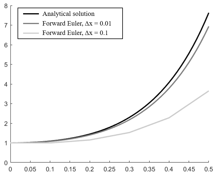This is best done using a coding software such as MATLAB or python, but excel can be used as well. Figure 2.4 shows a solution dataset using the Foward Euler approximation for $Δ x = . 1$ and $Δ x = . 01$ . The analytical ”ground truth” solution from equation 2.92 is provided as a comparison.

Figure 2.4: Forward Euler approximation for the solution dataset to equation 2.179 using a $Δ$ x of 0.1 and 0.01 as compared to the analytical solution provided in equation 2.92.

Example: PDE - The Heat Equation

We will use this section as an opportunity to provide a numerical solution set to the 2D version of the heat equation (the heat equation is derived in section ?? as equation ??). For continuity, the 2D heat equation is provided here as equation 2.185.

\begin{align} c_{p} ρ \frac{𝑑𝑇}{𝑑𝑡} = K \frac{d^{2} T}{d x^{2}} + K \frac{d^{2} T}{d y^{2}} & (2.185) \end{align}

For this example, we will assume that our 2D solid is a rectangle with a height of 50 and a width of 100. $c_{p}$ , $ρ$ and $K$ are constants that described in detail in section ??. In this example, these constants will be set to values as follows: $c_{p} = 1$ , $ρ = 1$ , $K = 5$ .

For our initial condition, we will assume that the entire solid is at a temperature of 100 at $t = 0$ . This is shown in equation 2.186.

\begin{align} T (x, y, 0) = 100 & (2.186) \end{align}

For our boundary conditions, we will assume that all edges have a temperature of 0 except for the right edge which is 200. This is shown in equation 2.187.

\begin{matrix} \begin{aligned} T (x, 0, t) & = 0 \\ T (x, L, t) & = 0 \\ T (0, y, t) & = 0 \\ T (L, y, t) & = 200 \end{aligned} \end{matrix}

(2.187)

Now, it is time to apply a finite difference approximation to equation 2.185. In this example, we will use forward difference (equation 2.162) for the $\frac{𝑑𝑇}{𝑑𝑡}$ term and second order central difference (equation 2.175) for the $\frac{d^{2} T}{d x^{2}}$ and $\frac{d^{2} T}{d y^{2}}$ terms. We will define our values at selected times $t_{k}$ , selected $x$ locations $x_{m}$ , and selected $y$ locations $y_{n}$ , where $k, m, n$ are integer values. To express $T$ at a given $t, x, y$ in a concise fashion, we will shorten $T (t_{k}, x_{m}, y_{n})$ to $T_{m, n}^{k}$ . Implementing this notation using our chosen finite different approximations, we get equation 2.188.

\begin{align} c_{p} ρ \frac{T_{m . n}^{k + 1} - T_{m . n}^{k}}{Δ t} = K \frac{T_{m + 1, n}^{k} - 2 T_{m, n}^{k} + T_{m - 1, n}^{k}}{Δ x^{2}} + K \frac{T_{m, n + 1}^{k} - 2 T_{m, n}^{k} + T_{m, n - 1}^{k}}{Δ y^{2}} & (2.188) \end{align}

Solving for $T_{m . n}^{k + 1}$ , we get equation 2.189.

\begin{align} T_{m . n}^{k + 1} = \frac{K Δ t}{c_{p} ρ Δ x^{2}} (T_{m + 1, n}^{k} - 2 T_{m, n}^{k} + T_{m - 1, n}^{k}) + \frac{K Δ t}{c_{p} ρ Δ y^{2}} (T_{m, n + 1}^{k} - 2 T_{m, n}^{k} + T_{m, n - 1}^{k}) + T_{m, n}^{k} & (2.189) \end{align}

Now, from our initial condition we know all of the $T_{m, n}^{0}$ points. Using equation 2.189, we can calculate all $T_{m, n}^{1}$ points. In this way, we can calculate the next time step points $T_{m, n}^{k + 1}$ based on $T_{m, n}^{k}$ by iteration at each timestep $k$ . This is best done in a coding software such as MATLAB or python. To provide the reader with a visualization of a solution to equation 2.185, equation 2.189 was input into a coding software to calculate temperature distribution of the rectangle for each time step. The result of numerical solution is shown in Figure 2.5 at select time steps 0, 20, 40, and 60. For the written code, increments were set as follows; $𝑑𝑥 = 𝑑𝑦 = 5$ , $𝑑𝑡 = . 5051$ .

Figure 2.5: Numerically computed solution to equation 2.185 at time steps 0, 20, 40, and 60.