Approximating Functions

2.5 Approximating Functions

This section is dedicated to methods of rewriting non-polynomial functions in a polynomial form. We will review two ways of doing this: the Taylor Series Expansion, and the Inner Product Method.

2.5.1 Taylor Series Expansion

The Taylor Series Expansion involves choosing constants of a polynomial in a manner that ensures that derivatives of said polynomial to the $𝑛𝑡h$ degree equal the non-polynomial function at a given point. As can be deduced, in order for this to work we must assume that our non-polynomial function can be written as a standard series with unknown constants. This assumption is shown in equation 2.238.

g (x) = C_{0} + C_{1} (x) + C_{2} {(x)}^{2} + . . . + C_{n} {(x)}^{n}

(2.238)

Our solution lies in finding the appropriate value for $C_{0}$ , $C_{1}$ , etc. In order to find $C_{0}$ , we can simply set $x = 0$ . Doing this, we get the equation 2.239.

g (0) = C_{0}

(2.239)

In order to find $C_{1}$ , we simply take the derivative of equation 2.238. Differentiating and again setting $x = 0$ , we get equation 2.240.

\frac{𝑑𝑔 (0)}{𝑑𝑥} = C_{1}

(2.240)

We can find $C_{2}$ by repeating the differentiating exercise and again setting $x = 0$ . Doing this we get equation 2.241.

\frac{1}{2} \frac{d^{2} g (0)}{d x^{2}} = C_{2}

(2.241)

If we repeat differentiation $n$ times, we will find that function $g (x)$ will be equal to equation 2.242.

g (x) = g (0) + \frac{𝑑𝑔 (0)}{𝑑𝑥} (x) + \frac{1}{2} \frac{d^{2} g (0)}{d^{2} x} x^{2} + \frac{1}{6} \frac{d^{3} g (0)}{d x^{3}} x^{3} + . . . + \frac{1}{n!} \frac{d^{n} g (0)}{𝑑𝑥} x^{n}

(2.242)

In equation 2.242, we were able to easily find our desired constants because we fixed our $x$ location at $x = 0$ . For this reason, we say that our polynomial approximation is centered at $x = 0$ . In order to center our polynomial approximation at arbitrary point $x = a$ , we start can start out with equation 2.243. This is a modified version of equation 2.238.

g (x) = C_{0} + C_{1} (x - a) + C_{2} {(x - a)}^{2} + . . . + C_{n} {(x - a)}^{n}

(2.243)

Finding the $C$ values using differentiation, we get equation 2.244.

g (x) = g (a) + \frac{𝑑𝑔 (a)}{𝑑𝑥} (x - a) + \frac{1}{2} \frac{d^{2} g (a)}{d^{2} x} {(x - a)}^{2} + \frac{1}{6} \frac{d^{3} g (a)}{d x^{3}} {(x - a)}^{3} + . . . + \frac{1}{n!} \frac{d^{n} g (a)}{𝑑𝑥} {(x - a)}^{n}

(2.244)

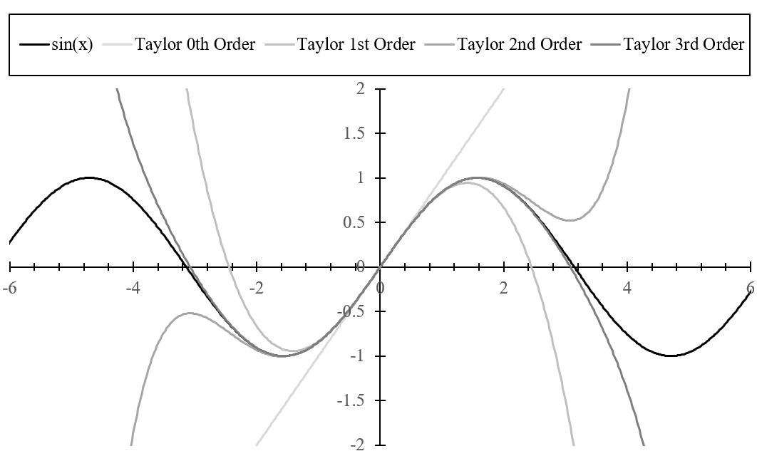
As can be easily deduced, our polynomial approximation for $g (x)$ is most accurate at $x = a$ (our function $g (x)$ and the polynomial approximation give exactly the same output at this point). The further away we get from $x = a$ , the more the output of our polynomial function diverges from the original non polynomial function $g (x)$ . In addition, the more terms we consider within our theoretically infinite polynomial approximation, the more accurate the polynomial approximation is at outputting an equivalent value as the original function. This phenomenon can be observed in Figure 2.8, which shows the function $y = \sin (x)$ along with a Taylor polynomial approximation (centered at $x = 0$ ) given different amounts of terms.

Figure 2.8: Graph showing the function $y = \sin (x)$ along with Taylor series approximations of varying order. Order corresponds to the amount of terms the Taylor polynomial goes out to; 0th order corresponds to one term, 1st to two terms, etc.

It is quite time consuming to calculate a Taylor Series of any non-polynomial function $g (x)$ . In order to shortcut this process, the Taylor approximations of common non-polynomial functions centered at $x = 0$ are provided in Table 2.4.

Table 2.4: Table showing common non-polynomial functions centered at

x = 0

$𝐲 = 𝐠 (𝐱)$	Taylor Series centered at $x = 0$



$\frac{1}{1 - x}$	$1 + x + x^{2} + x^{3} + . . . + x^{n}$

$e^{x}$	$1 + x + \frac{x^{2}}{2} + \frac{x^{3}}{3!} + \frac{x^{4}}{4!} + . . . + \frac{x^{n}}{n!}$

$\cos (x)$	$1 - \frac{x^{2}}{2} + \frac{x^{4}}{4!} - \frac{x^{6}}{6!} + . . . + {(- 1)}^{n} \frac{x^{2 n}}{(2 n)!}$

$\sin (x)$	$x - \frac{x^{3}}{3!} + \frac{x^{5}}{5!} - \frac{x^{7}}{7!} + . . . + {(- 1)}^{n} \frac{x^{2 n + 1}}{(2 n + 1)!}$

$\ln (1 + x)$	$x - \frac{x^{2}}{2} + \frac{x^{3}}{3} - \frac{x^{4}}{4} + . . . + {(- 1)}^{n + 1} \frac{x^{n}}{n}$

$\tan^{- 1} (x)$	$x - \frac{x^{3}}{3} + \frac{x^{5}}{5} - \frac{x^{7}}{7} + . . . . + {(- 1)}^{n} \frac{x^{2 n + 1}}{2 n + 1}$

Example: Euler’s Identity

In this example, we will generate a Taylor series approximation centered at $x = 0$ for the function provided in equation 2.245.

y = e^{𝑖𝑥}

(2.245)

In equation 2.245, $i$ is the imaginary number $\sqrt{- 1}$ introduced in section 2.8.3. Plugging equation 2.245 into equation 2.244 (assuming $a = 0$ ), we get equation 2.246.

e^{𝑖𝑥} = 1 + i (x) - \frac{1}{2} {(x)}^{2} - i \frac{1}{3!} x^{3} + \frac{1}{4!} x^{4} + i \frac{1}{5!} x^{5} - \frac{1}{6!} x^{6} - i \frac{1}{7!} x^{7} + . . .

(2.246)

We can regroup equation 2.246 as shown in equation 2.247.

e^{𝑖𝑥} = (1 - \frac{1}{2} {(x)}^{2} + \frac{1}{4!} x^{4} - \frac{1}{6!} x^{6} + . . .) + i (x - \frac{1}{3!} x^{3} + \frac{1}{5!} x^{5} - \frac{1}{7!} x^{7} + . . .) .

(2.247)

Now, you may notice from Table 2.4 that the left series in equation 2.247 is the Taylor series for $\cos (x)$ . The right series in equation 2.247 is the Taylor series for $\sin (x)$ . Therefore, we can rewrite equation 2.247 as shown in equation 2.248.

e^{𝑖𝑥} = \cos (x) + i \sin (x) .

(2.248)

Equation 2.248 is called Euler’s formula. Plugging in $x = π$ into equation 2.248, we are able to get Euler’s identify, shown in equation 2.249.

e^{𝑖𝜋} = 1

(2.249)

We can use a similar process as presented in this example to prove equation 2.250 is true.

e^{- 𝑖𝑥} = \cos (x) - i \sin (x) .

(2.250)

Expansion on Euler’s Identity

In this example, we will use above equations 2.248 and 2.250 to simplify equation 2.251.

y = A_{1} e^{(λ + 𝜇𝑖) x} + A_{2} e^{(λ - 𝜇𝑖) x}

(2.251)

Algebraically rewriting equation 2.251 and plugging in equations 2.248 and 2.250 we get equation 2.252.

y = (A_{1} + A_{2}) e^{𝜆𝑥} \cos (𝜇𝑥) + (A_{1} - A_{2}) i e^{𝜆𝑡} \sin (𝜇𝑥)

(2.252)

Now, we can define two constants as shown in equations 2.253 and 2.254.

\begin{align} C_{1} & = (A_{1} + A_{2}) & (2.253) \end{align}

\begin{align} C_{2} & = (A_{1} - A_{2}) i & (2.254) \end{align}

Plugging in equations 2.253 and 2.254 into equation 2.252 we are left with equation 2.255.

A_{1} e^{(λ + 𝜇𝑖) x} + A_{2} e^{(λ - 𝜇𝑖)} = C_{1} e^{𝜆𝑥} \cos (𝜇𝑥) + C_{2} e^{𝜆𝑥} \sin (𝜇𝑥)

(2.255)

2.5.2 Inner Product Approximation

The Inner Product Approximation is an alternative way to fit a polynomial function to a non-polynomial function. As in the Taylor series method, we start out with a standard polynomial to be fitted to a target function $g (x)$ . This “problem statement” is shown in equation 2.256.

g (x) = C_{0} + C_{1} (x) + C_{2} {(x)}^{2} + . . . + C_{n} {(x)}^{n}

(2.256)

Again, as with the Taylor Series Method, our solution lies with finding the appropriate values for $C_{0}$ , $C_{1}$ , etc. In the Taylor Series Method, it was possible to solve for $C_{0}$ , $C_{1}$ , etc. and then look for patterns. In this method, we need to decide from the start to which maximum value $n$ our fitting polynomial goes out to. Essentially, we need to start out with a finite term fitting function.

As the name of this method suggests, we will be using a mathematical construct called the inner product in order to find these values. The definition of the inner product between two functions $f (x)$ and $h (x)$ on the interval $[a, b]$ is provided in equation 2.257.

\int_{a}^{b} f (x) * h (x) 𝑑𝑥

(2.257)

The inner product can be thought of as analogous operator for continuous functions as the dot product (section 2.3.2) is for vectors. You may remember from the vectors section (section 2.3.2) that if the dot product of two vectors is 0, the vectors are considered orthogonal. In following this, equation 2.258 provides the definition of orthogonal functions $f (x)$ and $h (x)$ .

\int_{a}^{b} f (x) * h (x) 𝑑𝑥 = 0

(2.258)

Given equation 2.258, we can make a mental extrapolation to the curve fitting methodology presented in section 2.4. As a reminder, in this procedure, our target modeling function provided us with vectors within a given vector space (shown in equation 2.207). We used the Gram-Schmidt Orthogonalization Procedure to orthogonalize the vectors within this vector space with the goal of deriving an orthogonal basis. We then projected the given vector $\vec{y}$ onto this new vector space (shown in equation 2.209). Within the process of projecting, we got the closest vector to $\vec{y}$ that exists within this vector space (this closest vector is defined within section 2.4 as ${\vec{y}}_{f}$ ). Our mental extrapolation consists of thinking of our target modeling function (equation 2.256) as a span of functions { $1$ , $x$ , $x^{2}$ , ..., $x^{n}$ }. We are trying to find the combination of functions within this span that makes this span best fit our given function $g (x)$ on the interval $[a, b]$ (although I am using slightly different terminology here to drive the connection between function fitting and curve fitting, this best fit manifests itself in simply finding the correct $C_{0}$ , $C_{1}$ , etc). Therefore, we can follow the general procedure laid out in section 2.4, but tweak it for functions (replace every dot product with an inner product). Our first step is to derive a set of orthogonal functions { $e_{1}$ , $e_{2}$ ,..., $e_{n}$ } for our span of functions. We can do this my mimicking the Gram-Schmidt Orthogonalization Procedure out to desired function $x^{n}$ as shown in the following sequence.

\begin{array}{l} e_{1} & = 1 \\ e_{2} & = x - \frac{\int_{a}^{b} e_{1} * 𝑥𝑑𝑥}{\int_{a}^{b} e_{1} * e_{1} 𝑑𝑥} e_{1} \\ e_{3} & = x^{2} - \frac{\int_{a}^{b} e_{2} * x^{2} 𝑑𝑥}{\int_{a}^{b} e_{2} * e_{2} 𝑑𝑥} e_{2} - \frac{\int_{a}^{b} e_{1} * x^{2} 𝑑𝑥}{\int_{a}^{b} e_{1} * e_{1} 𝑑𝑥} e_{1} \\ e_{n} & = . . . \end{array}

In following the curve fitting procedure, our next step is to project our given function $g (x)$ onto our derived orthogonal set of functions. We can do this my mimicking equation 2.209 for functions as shown in equation 2.259.

\begin{align} \frac{\int_{a}^{b} e_{1} * g (x) 𝑑𝑥}{\int_{a}^{b} e_{1} * e_{1} 𝑑𝑥} e_{1} + \frac{\int_{a}^{b} e_{2} * g (x) 𝑑𝑥}{\int_{a}^{b} e_{2} * e_{2} 𝑑𝑥} e_{2} + \frac{\int_{a}^{b} e_{3} * g (x) 𝑑𝑥}{\int_{a}^{b} e_{3} * e_{3} 𝑑𝑥} e_{3} + . . . + \frac{\int_{a}^{b} e_{n} * g (x) 𝑑𝑥}{\int_{a}^{b} e_{n} * e_{n} 𝑑𝑥} e_{n} & (2.259) \end{align}

In doing this, we will get a polynomial with coefficients. We have essentially found the points $C_{1}$ , $C_{2}$ , etc. that cause our original function (equation 2.256) to most closely match $g (x)$ on the given interval $[a, b]$ .

Short Example

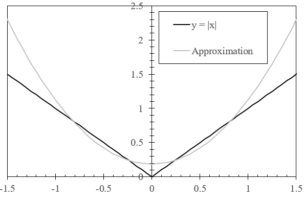
In this example, we will fit the equation $g (x) = | x |$ to a polynomial. We will limit our fitting polynomial to the first 3 terms of the general equation provided in 2.256 on the interval $[- 1, 1]$ . Therefore, our problem statement resembles equation 2.260.

\begin{align} | x | = C_{0} + C_{1} x + C_{2} x^{2} & (2.260) \end{align}

Our goal is to find $C_{0}$ , $C_{1}$ , and $C_{2}$ that make this as true as possible. Our modeling function span is ${1, x, x^{2}}$ . Our first step is orthogonalize these functions using the Gram-Schmidt Orthogoanliztaion Procedure for functions laid out previously. Doing this, we get the following orthogonal function basis.

\begin{array}{l} e_{1} & = 1 \\ e_{2} & = x \\ e_{3} & = x^{2} - \frac{1}{3} \end{array}

Now we simply project $| x |$ onto the orthogonal basis using equation 2.259. Doing this, we get equation 2.261.

\begin{align} | x | \approx \frac{15}{16} x^{2} + 3 ∕ 16 & (2.261) \end{align}

The function $| x |$ along with the polynomial approximation shown in equation 2.261 is shown in Figure 2.9.

Figure 2.9: Graph showing the function $y = | x |$ along with the 2nd order inner product approximation shown in equation 2.261