Matrices

2.6 Matrices

Matrices are mathematical entities consisting of specifically ordered groups of numbers. An example of a matrix is shown in expression 2.262.

[\begin{matrix} a_{11} & a_{12} & a_{13} \\ a_{21} & a_{22} & a_{23} \\ a_{31} & a_{32} & a_{33} \end{matrix}]

(2.262)

Matrix 2.262 is considered a 3 x 3 size matrix because it has 3 rows and 3 columns. Please note that when specifying the size of matrix, the number of rows always comes first ( $i$ rows x $j$ columns). This convention extends to the subscripts of our inner-matrix terms; at location row 2 column 1 we have $a_{12}$ .

A number of specific operations can be performed on matrices. The ability to perform said operations typically depends on the size of the given matrix (or matrices). We will cover the most common matrix operations in the following sections.

Matrix Addition

Matrices can be added as shown in equation 2.263.

[\begin{matrix} a_{11} & a_{12} & a_{13} & . . . & a_{1 j} \\ a_{21} & a_{22} & a_{23} & . . . & a_{2 j} \\ a_{31} & a_{32} & a_{33} & . . . & a_{3 j} \\ . & . & . \\ . & . & . \\ . & . & . \\ a_{i 1} & a_{i 2} & a_{i 3} \end{matrix}] + [\begin{matrix} b_{11} & b_{12} & b_{13} & . . . & b_{1 j} \\ b_{21} & b_{22} & b_{23} & . . . & b_{2 j} \\ b_{31} & b_{32} & b_{33} & . . . & b_{3 j} \\ . & . & . \\ . & . & . \\ . & . & . \\ b_{i 1} & b_{i 2} & b_{i 3} \end{matrix}] = [\begin{matrix} a_{11} + b_{11} & a_{12} + b_{12} & a_{13} + b_{13} & . . . & a_{1 j} + b_{1 j} \\ a_{21} + b_{21} & a_{22} + b_{22} & a_{23} + b_{23} & . . . & a_{2 j} + b_{2 j} \\ a_{31} + b_{31} & a_{32} + b_{32} & a_{33} + b_{33} & . . . & a_{3 j} + b_{3 j} \\ . & . & . \\ . & . & . \\ . & . & . \\ a_{i 1} + b_{i 1} & a_{i 2} + b_{i 2} & a_{i 3} + b_{i 3} \end{matrix}]

(2.263)

Only matrices of the same size can be added.

Scalar Multiplication

A matrix can be multiplied by a scalar $(k)$ as shown in equation 2.264.

k * ([\begin{matrix} a_{11} & a_{12} & a_{13} & . . . & a_{1 j} \\ a_{21} & a_{22} & a_{23} & . . . & a_{2 j} \\ a_{31} & a_{32} & a_{33} & . . . & a_{3 j} \\ . & . & . \\ . & . & . \\ . & . & . \\ a_{i 1} & a_{i 2} & a_{i 3} \end{matrix}]) = [\begin{matrix} k * a_{11} & k * a_{12} & k * a_{13} & . . . & k * a_{1 j} \\ k * a_{21} & k * a_{22} & k * a_{23} & . . . & k * a_{2 j} \\ k * a_{31} & k * a_{32} & k * a_{33} & . . . & k * a_{3 j} \\ . & . & . \\ . & . & . \\ . & . & . \\ k * a_{i 1} & k * a_{i 2} & k * a_{i 3} \end{matrix}]

(2.264)

There are no limitations on the size of matrices that be multiplied by a scalar.

Matrix Multiplication

Matrix multiplications derives its logic from coordinate system transformations. However, since this is not a mathematics book, we will not go into covering the motivation for matrix multiplication convention. Rather, simply the methodology will be presented.

Unlike scalar multiplication, the order in which two matrices are multiplied matters. The output matrix is calculated by taking the dot product of the columns in the first matrix with the rows in the second matrix. As can be deduced from the previous sentence, this means that the number of columns in the first matrix must match the number of rows in the second matrix. Generalized matrix multiplication is shown in equation 2.265.

[\begin{matrix} a_{11} & a_{12} & . . . & a_{1 j} \\ a_{21} & a_{22} & . . . & a_{2 j} \\ . & . \\ . & . \\ . & . \\ a_{i 1} & a_{i 2} \end{matrix}] * [\begin{matrix} b_{11} & b_{12} & . . . & b_{1 n} \\ b_{21} & b_{22} & . . . & b_{2 n} \\ . & . \\ . & . \\ . & . \\ b_{m 1} & b_{m 2} \end{matrix}] = [\begin{matrix} a_{11} b_{11} + a_{12} b_{21} & a_{11} b_{12} + a_{12} b_{22} & a_{11} b_{13} + a_{12} b_{23} & . . . \\ a_{21} b_{11} + a_{22} b_{21} & a_{21} b_{12} + a_{22} b_{22} & a_{21} b_{13} + a_{22} b_{23} & . . . \\ . & . \\ . & . \\ . & . \end{matrix}]

(2.265)

As can be observed, we multiplied $i$ x $j$ matrix $A$ with $m$ x $n$ matrix $B$ . Given that $j$ must equal $m$ , our result is a $i$ x $n$ matrix.

Transposition

The transpose of a matrix is accomplished by switching the rows and columns of a matrix as shown in equation 2.266.

{([\begin{matrix} a_{11} & a_{12} & a_{13} & . . . & a_{1 j} \\ a_{21} & a_{22} & a_{23} & . . . & a_{2 j} \\ a_{31} & a_{32} & a_{33} & . . . & a_{3 j} \\ . & . & . \\ . & . & . \\ . & . & . \\ a_{i 1} & a_{i 2} & a_{i 3} \end{matrix}])}^{T} = [\begin{matrix} a_{11} & a_{21} & a_{31} & . . . & a_{i 1} \\ a_{12} & a_{22} & a_{32} & . . . & a_{i 2} \\ a_{13} & a_{23} & a_{33} & . . . & a_{i 3} \\ . & . & . \\ . & . & . \\ . & . & . \\ a_{1 j} & a_{2 j} & a_{3 j} \end{matrix}]

(2.266)

As can be deduced, any size matrix can be transposed.

Some properties associated with transposed matrices are provided in equations 2.267, 2.268, 2.269, and 2.270.

{({[A]}^{T})}^{T} = [A]

(2.267)

{([A] [B])}^{T} = {[B]}^{T} {[A]}^{T}

(2.268)

{([A] + [B])}^{T} = {[A]}^{T} + {[B]}^{T}

(2.269)

{([A] [B] [C])}^{T} = {[C]}^{T} {[B]}^{T} {[A]}^{T}

(2.270)

Determinant

A determinant of a matrix is a number that is calculated from a matrix. The determinant of a 2 x 2 matrix is calculated as shown in equation 2.271.

𝑑𝑒𝑡 ([\begin{matrix} a_{11} & a_{12} \\ a_{21} & a_{22} \end{matrix}]) = a_{11} a_{22} - a_{12} a_{21}

(2.271)

The determinant of a 3 x 3 matrix is calculated as shown in equation 2.272.

𝑑𝑒𝑡 ([\begin{matrix} a_{11} & a_{12} & a_{13} \\ a_{21} & a_{22} & a_{23} \\ a_{31} & a_{32} & a_{33} \end{matrix}]) = a_{11} (a_{22} a_{33} - a_{23} a_{32}) - a_{12} (a_{21} a_{33} - a_{23} a_{31}) + a_{31} (a_{21} a_{32} - a_{22} a_{31})

(2.272)

It is possible to find the determinant of larger square matrices. However, the methodology for this is not covered in this book.

As will be reviewed in the inverse section, a matrix can only be inverted if it has a nonzero determinant.

Cofactor Matrix

The cofactor matrix is a new matrix that can be calculated from a given square matrix. Within this section, we will review how to calculate a cofactor matrix only for 3 x 3 matrix. A sample 3 x 3 matrix is provided in equation 2.273.

[\begin{matrix} a_{11} & a_{12} & a_{13} \\ a_{21} & a_{22} & a_{23} \\ a_{31} & a_{32} & a_{33} \end{matrix}]

(2.273)

The co-factor matrix of matrix 2.273 is symbolized by matrix 2.274.

[\begin{matrix} C_{11} & C_{12} & C_{13} \\ C_{21} & C_{22} & C_{23} \\ C_{31} & C_{32} & C_{33} \end{matrix}]

(2.274)

Each corresponding $C$ term is calculated by finding the determinant of the 4 other matrix terms not included in the target term row or column. The following equations show this for all $C$ values in matrix 2.274.

C_{11} = 𝑑𝑒𝑡 ([\begin{matrix} a_{22} & a_{23} \\ a_{32} & a_{33} \end{matrix}])

C_{12} = - 𝑑𝑒𝑡 ([\begin{matrix} a_{21} & a_{23} \\ a_{31} & a_{33} \end{matrix}])

C_{13} = 𝑑𝑒𝑡 ([\begin{matrix} a_{21} & a_{22} \\ a_{31} & a_{32} \end{matrix}])

C_{21} = - 𝑑𝑒𝑡 ([\begin{matrix} a_{12} & a_{13} \\ a_{32} & a_{33} \end{matrix}])

C_{22} = 𝑑𝑒𝑡 ([\begin{matrix} a_{11} & a_{13} \\ a_{31} & a_{33} \end{matrix}])

C_{23} = - 𝑑𝑒𝑡 ([\begin{matrix} a_{11} & a_{12} \\ a_{31} & a_{32} \end{matrix}])

C_{31} = 𝑑𝑒𝑡 ([\begin{matrix} a_{12} & a_{13} \\ a_{22} & a_{23} \end{matrix}])

C_{32} = - 𝑑𝑒𝑡 ([\begin{matrix} a_{11} & a_{13} \\ a_{21} & a_{23} \end{matrix}])

C_{33} = 𝑑𝑒𝑡 ([\begin{matrix} a_{11} & a_{12} \\ a_{21} & a_{22} \end{matrix}])

Please note that some of co-factor matrix terms have a selectively placed coefficient negative.

Inverse

The inverse of example matrix $[A]$ is referred to as ${[A]}^{- 1}$ . Its definition is shown in equation 2.275.

[A] * {[A]}^{- 1} = [\begin{matrix} 1 & 0 & 0 & . . . \\ 0 & 1 & 0 & . . . \\ 0 & 0 & 1 & . . . \\ . & . & . \\ . & . & . \\ . & . & . \end{matrix}]

(2.275)

Not all matrices are invertable. The matrix to the right hand side in equation 2.275 is called the identity matrix, and within this book will be symbolized as $[I]$ . The identity matrix is always square ( $i = j$ ) and has a value of 1 in the diagonal indices, along with 0 in all other indices. As can be deduced, for a matrix to have an inverse it must be square. There are two methods to finding the inverse of a matrix; the Gauss Jordan Elimination method and the adjoint method. They will be presented using an example 3 x 3 matrix.

The Gauss Jordan Elimination method involves starting with the set up shown in expression 2.276.

[\begin{matrix} a_{11} & a_{12} & a_{13} & | & 1 & 0 & 0 \\ a_{21} & a_{22} & a_{23} & | & 0 & 1 & 0 \\ a_{31} & a_{32} & a_{33} & | & 0 & 0 & 1 \end{matrix}]

(2.276)

The subsequent rows are multiplied by scalars and added to each other with the goal of making the left hand side of expression 2.276 become the identity matrix $[I]$ . When this occurs, the right hand side of expression 2.276 will be ${[A]}^{- 1}$ .

The adjoint method involves calculating the inverse of a matrix using equation 2.277.

A^{- 1} = \frac{1}{𝑑𝑒𝑡 ([A])} {[C]}^{T}

(2.277)

In equation 2.277, $[C]$ is the cofactor matrix (the method of calculating this matrix was explained previously) of original matrix $[A]$ .

The method of finding the cofactor matrix was within this book only presented for a 3 x 3 matrix. For a 2 x 2 matrix, the equation 2.277 can be rewritten as shown in equation 2.278.

{[A]}^{- 1} = \frac{1}{𝑑𝑒𝑡 ([A])} [\begin{matrix} a_{22} & - a_{21} \\ - a_{12} & a_{11} \end{matrix}]

(2.278)

2.6.1 Eigenvalues and Eigenvectors

A vector (section 2.3) of $a_{1} î + a_{2} ĵ + a_{3} \hat{k} + . . . + a_{i} ẑ$ form can be expressed as a matrix as shown in equation 2.279.

[\begin{matrix} a_{1} \\ a_{2} \\ a_{3} \\ . \\ . \\ . \\ a_{i} \end{matrix}]

(2.279)

Essentially, vectors can be thought of as column matrices with dimensions of ( $i$ , 1) where $i$ is the number of basis vectors in the given vector space ( $i$ should not be confused with $î$ , which is simply a basis vector as specified in section 2.3). If we multiply an input vector $[a]$ (in matrix form) of dimension ( $i$ , 1) by a matrix $[b]$ of dimension $(i, i)$ we will get an output vector $[c]$ of dimension ( $i$ , 1). This is shown in equation 2.280.

[\begin{matrix} c_{1} \\ c_{2} \\ c_{3} \\ . \\ . \\ . \\ c_{i} \end{matrix}] = [\begin{matrix} b_{11} & b_{12} & b_{13} & . . . & b_{1 j} \\ b_{21} & b_{22} & b_{23} & . . . & b_{2 j} \\ b_{31} & b_{32} & b_{33} & . . . & b_{3 j} \\ . & . & . \\ . & . & . \\ . & . & . \\ b_{i 1} & b_{i 2} & b_{i 3} \end{matrix}] * [\begin{matrix} a_{1} \\ a_{2} \\ a_{3} \\ . \\ . \\ . \\ a_{i} \end{matrix}]

(2.280)

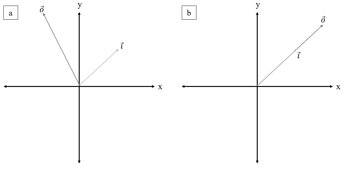
For this reason, matrices can be thought of operating onto vectors, and are commonly referred to as operators. In most cases, the input vector $\vec{i}$ will be linearly independent of the output vector $\vec{o}$ for a given matrix as shown in Figure 2.10a. However, depending on the matrix a specific $\vec{i}$ can output a $\vec{o}$ which is a scalar multiple of $\vec{i}$ (i.e. $\vec{o}$ is proportional to and acts in the same direction as $\vec{i}$ ). This is shown in Figure 2.10b. When this happens, the $\vec{i}$ is referred to as a eigenvector. The ratio $\frac{| | \vec{o} | |}{| | \vec{i} | |}$ is referred to as a eigenvalue.

Figure 2.10: Graph showing the input vector $\vec{i}$ and output vector $\vec{o}$ for a given 2x2 matrix. (a) shows a scenario $\vec{o}$ is linearly independent of $\vec{i}$ . (b) shows an $\vec{o}$ which is linearly dependent on $\vec{i}$ ; $\vec{i}$ is an eigenvector.

Our task is to find eigenvectors and their corresponding eigenvalues for a given matrix $[B]$ . This problem is shown mathematically in equation 2.281.

[B] * \vec{v} = λ \vec{v}

(2.281)

In equation 2.281, $\vec{v}$ is the eigenvector, and $λ$ is the eigenvalue. Subtracting $λ \vec{v}$ from both sides, we get equation 2.282.

[B] * \vec{v} - λ \vec{v} = 0

(2.282)

However, following the rules of section 2.6.0.0, the dimensions of $[B] * \vec{v}$ and $λ \vec{v}$ do not match, meaning that we cannot add them. Luckily for us, we can make $λ \vec{v}$ have matching dimensions by multiplying by the identity matrix $[I]$ (explained in section 2.6.0.0).

[B] * \vec{v} - λ [I] \vec{v} = 0

(2.283)

Factoring out $\vec{v}$ , we get equation 2.284.

([B] - λ [I]) \vec{v} = 0

(2.284)

Multiplying both sides by ${([B] - λ [I])}^{- 1}$ , we get equation 2.285.

{([B] - λ [I])}^{- 1} ([B] - λ [I]) \vec{v} = 0

(2.285)

From the zero product property, we know that either ${([B] - λ [I])}^{- 1} ([B] - λ [I])$ or $\vec{v}$ must equal 0. From section 2.6.0.0 we know that ${([B] - λ [I])}^{- 1} ([B] - λ [I]) = 1$ . So, this would force $\vec{v} = 0$ . However, we are looking for non-zero eigenvectors! So, we can state that we are interested in eigenvectors where ${([B] - λ [I])}^{- 1} ([B] - λ [I]) \neq 1$ , which means we are looking for solutions where $([B] - λ [I])$ is not invertable. As reviewed in section 2.6.0.0 a matrix is not invertable if its determinant (section 2.6.0.0) is equal to 0. Therefore, we can solve for eigenvalues $λ$ using equation 2.286.

𝑑𝑒𝑡 ([B] - λ [I]) = 0

(2.286)

It is possible to get anywhere between $i$ and 0 eigenvalues for a matrix of dimensions ( $i, i$ ). The eigenvector can be found by solving equation 2.287 for each eigenvalue $λ$ .

([B] - λ_{n} [I]) \vec{v_{n}} = 0

(2.287)

In equation 2.287, the $n$ subscript in $λ_{n}$ and ${\vec{v}}_{n}$ indicates that the eigenvalue ${\vec{v}}_{n}$ corresponds to eigenvalue $λ_{n}$ .

The eigenvalues for a matrix can be expressed as a diagonal form as shown in equation 2.288.

[λ] = [\begin{matrix} λ_{1} & 0 & . . . & 0 \\ 0 & λ_{2} & . . . & 0 \\ . & . \\ . & . \\ . & . \\ 0 & 0 & . . . & λ_{i} \end{matrix}]

(2.288)

The eigenvectors for a given matrix can be expressed in matrix form by stacking the eigenvectors horizontally as shown in equation 2.289.

[V] = [\vec{v_{1}}, \vec{v_{2}}, . . ., \vec{v_{n}}]

(2.289)

An interesting property of eigenvalues and eigenvectors lies in the fact that original matrix $[B]$ multiplied by its $[V]$ is equal to $[λ]$ multiplied by $[V]$ . This is shown in equation 2.290.

[B] [V] = [V] [λ]

(2.290)

We can multiply both sides of equation 2.290 by ${[V]}^{- 1}$ to obtain equation 2.291.

[B] = [V] [λ] {[V]}^{- 1}

(2.291)

Expressing $[B]$ in the form shown in equation 2.291 is referred to as diagonalizing the matrix.

The concept of eigenvalues and eigenvectors is critical to understanding the engineering concepts of principle moments of inertia (section ??) and principle stress directions (section ??).