Curve Fitting

2.4 Curve Fitting

The goal of this section is to derive a method which we can use to generate a best fit function $g (x)$ for given points $(x_{1}, y_{1}), (x_{2}, y_{2}), (x_{3}, y_{3}), . . . ., (x_{n}, y_{n})$ . One constraint with the process presented in this section is that our best fit function $g (x)$ must be of the form $c_{1} f_{1} (x) + c_{2} f_{2} (x) + c_{3} f_{3} (x) + . . . + c_{n} f_{n} (x)$ . Our first step in deriving a method to find the desired best fit function is to understand a vector process called the Gram-Schmidt Orthogonalization procedure.

Introduction to the Gram-Schmidt Orthogonalization Procedure

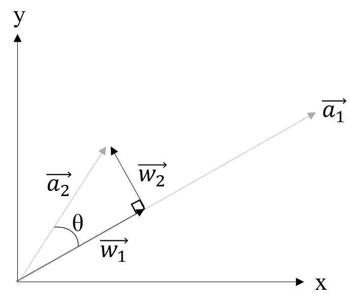
The goal of the Gram-Schmidt Orthogonalization procedure is to find a set of orthogonal vectors (section 2.3.2) which exist in the same vector space as defined by a given set of vectors. In order to do this, we will use Figure 2.6. ${\vec{a}}_{1}$ and ${\vec{a}}_{2}$ are arbitrary vectors which exist in a common vector space. ${\vec{w}}_{1}$ is the component of ${\vec{a}}_{2}$ that exists in the vector space with a basis defined by just ${\vec{a}}_{1}$ . ${\vec{w}}_{2}$ is orthogonal to ${\vec{w}}_{1}$ . Our goal is to find mathematical expressions for ${\vec{w}}_{1}$ and ${\vec{w}}_{2}$ .

Figure 2.6: Vectors used for the derivation of the Gram-Schmidt Orthogonalization procedure

Let us start with ${\vec{w}}_{1}$ . Using geometry, we can state equation 2.202.

\begin{align} {\vec{w}}_{1} = | | {\vec{a}}_{2} | | \cos 𝜃 * \frac{{\vec{a}}_{1}}{| | {\vec{a}}_{1} | |} & (2.202) \end{align}

Plugging in equation 2.197 for $\cos 𝜃$ , we get equation 2.203.

\begin{align} {\vec{w}}_{1} = | | {\vec{a}}_{2} | | * \frac{{\vec{a}}_{1} \cdot {\vec{a}}_{2}}{| | {\vec{a}}_{1} | | * | | {\vec{a}}_{2} | |} * \frac{{\vec{a}}_{1}}{| | {\vec{a}}_{1} | |} & (2.203) \end{align}

Simplifying equation 2.203 and plugging in the relation that $| | {\vec{a}}_{1} | | * | | {\vec{a}}_{1} | | = {\vec{a}}_{1} \cdot {\vec{a}}_{1}$ we are left with equation 2.204.

\begin{align} {\vec{w}}_{1} = \frac{{\vec{a}}_{2} \cdot {\vec{a}}_{1}}{{\vec{a}}_{1} \cdot {\vec{a}}_{1}} {\vec{a}}_{1} & (2.204) \end{align}

Now, we know that ${\vec{w}}_{2}$ is simply equal to ${\vec{a}}_{2} - {\vec{w}}_{1}$ . ${\vec{w}}_{2}$ is orthogonal to both ${\vec{a}}_{1}$ and ${\vec{w}}_{1}$ . Therefore, the vectors ${\vec{a}}_{1}$ and ${\vec{w}}_{2}$ constitute a set of orthogonal vectors that exist within the same vector space as the original ${\vec{a}}_{1}$ and ${\vec{a}}_{2}$ . We have achieved our goal. We can extend this methodology to find an orthogonal vectors ${\vec{u}}_{1}, {\vec{u}}_{2}, . . ., {\vec{u}}_{n}$ within the same vector space as input vectors ${\vec{a}}_{1}, \vec{a_{2}}, . . . {\vec{a}}_{n}$ . This is shown in the following equation.

\begin{array}{l} {\vec{u}}_{1} & = {\vec{a}}_{1} \\ {\vec{u}}_{2} & = {\vec{a}}_{2} - \frac{{\vec{u}}_{1} \cdot {\vec{a}}_{2}}{{\vec{u}}_{1} \cdot {\vec{u}}_{1}} {\vec{u}}_{1} \\ {\vec{u}}_{3} & = {\vec{a}}_{3} - \frac{{\vec{u}}_{1} \cdot {\vec{a}}_{3}}{{\vec{u}}_{1} \cdot {\vec{u}}_{1}} {\vec{u}}_{1} - \frac{{\vec{u}}_{2} \cdot {\vec{a}}_{3}}{{\vec{u}}_{2} \cdot {\vec{u}}_{2}} {\vec{u}}_{2} \\ {\vec{u}}_{n} & = . . . \end{array}

In the general equations provided, ${\vec{u}}_{2}$ is equal to the ${\vec{w}}_{2}$ shown in Figure 2.6. The big picture concept of the presented procedure is to force ${\vec{u}}_{n + 1}$ to be orthogonal to ${\vec{u}}_{n}$ by subtracting out components of ${\vec{a}}_{n + 1}$ that are not orthogonal. This process can be repeated as many times as necessary to generate a full orthogonal set $u_{1}, u_{2}, . . ., u_{n}$ .

Using the Gram-Schmidt Orthogonalization Procedure for Curve Fitting

As mentioned previously, for the method presented in this section, our best fit function must be of the form shown in equation 2.205.

\begin{align} c_{1} f_{1} (x) + c_{2} f_{2} (x) + c_{3} f_{3} (x) + . . . + c_{n} f_{n} (x) = y & (2.205) \end{align}

Plugging a given dataset $(x_{1}, y_{1}), (x_{2}, y_{2}), (x_{3}, y_{3}), . . ., (x_{n}, y_{n})$ into equation 2.205, we get equation 2.206.

c_{1} [\begin{matrix} f_{1} (x_{1}) \\ f_{1} (x_{2}) \\ f_{1} (x_{3}) \\ f_{1} (x_{n}) \end{matrix}] + c_{2} [\begin{matrix} f_{2} (x_{1}) \\ f_{2} (x_{2}) \\ f_{2} (x_{3}) \\ f_{2} (x_{n}) \end{matrix}] + c_{3} [\begin{matrix} f_{3} (x_{1}) \\ f_{3} (x_{2}) \\ f_{3} (x_{3}) \\ f_{3} (x_{n}) \end{matrix}] + c_{n} [\begin{matrix} f_{n} (x_{1}) \\ f_{n} (x_{2}) \\ f_{n} (x_{3}) \\ f_{n} (x_{n}) \end{matrix}] \approx [\begin{matrix} y_{1} \\ y_{2} \\ y_{3} \\ y_{n} \end{matrix}]

(2.206)

Essentially, the trick is to chose the correct $c_{1}, c_{2}, c_{3}, . . ., c_{n}$ so that our $\approx$ is as close as possible to the given $y_{1}, y_{2}, y_{3}, . . ., y_{n}$ . Please note that I have transitioned from using the $⟨$ $⟩$ notation for vectors and instead have shifted to large brackets in order to present the above equation in a more intuitive form. In moving forward with this vector mindset, we will refer the vector with coefficient $c_{1}$ as ${\vec{a}}_{1}$ . This logic can be extrapolated to ${\vec{a}}_{n}$ , while the vector with components of $y_{1}, y_{2}, y_{3}, . . ., y_{n}$ will be referred to as $\vec{y}$ . This is shown mathematically in equation 2.207.

\begin{align} c_{1} {\vec{a}}_{1} + c_{2} {\vec{a}}_{2} + c_{3} {\vec{a}}_{3} + . . . + c_{n} {\vec{a}}_{n} \approx \vec{y} & (2.207) \end{align}

You may notice that ${\vec{a}}_{1}, {\vec{a}}_{2}, {\vec{a}}_{3}, . . ., {\vec{a}}_{n}$ can be thought of as constituting a vector space.

In order to find the desired $c_{1} . c_{2}, c_{3}, . . ., c_{n}$ we first start out by building an orthogonal basis for the vector space defined by equation 2.207. In order to do this, we can use the gram-schmidt orthogonalization procedure explained previously to transform ${\vec{a}}_{1}, {\vec{a}}_{2}, {\vec{a}}_{3}, . . ., {\vec{a}}_{n}$ to the orthogonal counterparts ${\vec{u}}_{1}, {\vec{u}}_{2}, . . ., {\vec{u}}_{n}$ . We then want to find the vector that exists within this basis that is “closest” to $\vec{y}$ . This vector will be defined as ${\vec{y}}_{f}$ . Mathematically, we can state that we have found the correct ${\vec{y}}_{f}$ when the dot product of the difference between $\vec{y}$ and ${\vec{y}}_{f}$ ( $\vec{w}$ ) with $\vec{y}$ is 0. If this is confusing, reference Figure 2.6, and imagine ${\vec{a}}_{1}$ is vector basis of ${\vec{y}}_{f}$ , while ${\vec{a}}_{2}$ is our true $y$ . Thus, we state the closest any vector within the vector space of ${\vec{a}}_{1}$ can get to ${\vec{a}}_{2}$ is a ${\vec{y}}_{f}$ such that ${\vec{y}}_{f} \cdot (\vec{y} - {\vec{y}}_{f}) = 0$ . $(\vec{y} - {\vec{y}}_{f})$ is ${\vec{w}}_{2}$ in Figure 2.6. Thus, we get equation 2.208.

\begin{align} {\vec{y}}_{f} \cdot (\vec{y} - {\vec{y}}_{f}) = 0 & (2.208) \end{align}

We can use equation 2.204 to find ${\vec{y}}_{f}$ for ${\vec{u}}_{1}, {\vec{u}}_{2}, . . ., {\vec{u}}_{n}$ as shown in equation 2.209.

\begin{align} \frac{\vec{y} \cdot {\vec{u}}_{1}}{{\vec{u}}_{1} \cdot {\vec{u}}_{1}} {\vec{u}}_{1} + \frac{\vec{y} \cdot {\vec{u}}_{2}}{{\vec{u}}_{2} \cdot {\vec{u}}_{2}} {\vec{u}}_{2} + . . . . + \frac{\vec{y} \cdot {\vec{u}}_{n}}{{\vec{u}}_{n} \cdot {\vec{u}}_{n}} {\vec{u}}_{n} = {\vec{y}}_{f} & (2.209) \end{align}

Since $y_{f}$ is build up from vectors that exist within our original vector space ( ${\vec{a}}_{1}, {\vec{a}}_{2}, {\vec{a}}_{3}, . . ., {\vec{a}}_{n}$ ), we know that there exists a combination of $c_{1}, c_{2}, . . ., c_{n}$ that output this vector. These values are the solution to our problem. Therefore, we can use system of equation techniques to solve equation 2.210 and obtain our coefficients of interest.

c_{1} [\begin{matrix} f_{1} (x_{1}) \\ f_{1} (x_{2}) \\ f_{1} (x_{3}) \\ f_{1} (x_{n}) \end{matrix}] + c_{2} [\begin{matrix} f_{2} (x_{1}) \\ f_{2} (x_{2}) \\ f_{2} (x_{3}) \\ f_{2} (x_{n}) \end{matrix}] + c_{3} [\begin{matrix} f_{3} (x_{1}) \\ f_{3} (x_{2}) \\ f_{3} (x_{3}) \\ f_{3} (x_{n}) \end{matrix}] + c_{n} [\begin{matrix} f_{n} (x_{1}) \\ f_{n} (x_{2}) \\ f_{n} (x_{3}) \\ f_{n} (x_{n}) \end{matrix}] = {\vec{y}}_{f}

(2.210)

Using Matrix Techniques

The process presented in the previous section requires a considerable amount of work. First, $y_{f}$ must be found. Later, a system of equations needs to be solved for $c_{1}, c_{2}, c_{3}, . . ., c_{n}$ . In this section, we will derive a matrix (section 2.6) process for finding $c_{1}, c_{2}, c_{3}, . . ., c_{n}$ . The first step in doing this is to recognize that ${\vec{u}}_{k} \cdot \vec{y}$ can be rewritten as ${[u_{k}]}^{T} [y]$ (therefore transforming ${\vec{u}}_{k}$ as a 1x3 matrix and $\vec{y}$ as a 3x1 matrix). Given this, we can rewrite equation 2.209 as shown in equation 2.211.

\begin{align} \frac{1}{{\vec{u}}_{1} \cdot {\vec{u}}_{1}} [u_{1}] {[u_{1}]}^{T} [y] + \frac{1}{{\vec{u}}_{2} \cdot {\vec{u}}_{2}} [u_{2}] {[u_{2}]}^{T} [y] + . . . . + \frac{1}{{\vec{u}}_{n} \cdot {\vec{u}}_{n}} [u_{n}] {[u_{n}]}^{T} [y] = {\vec{y}}_{f} & (2.211) \end{align}

We can factor out $[y]$ from equation 2.211 as shown in equation 2.212.

\begin{align} [\frac{1}{{\vec{u}}_{1} \cdot {\vec{u}}_{1}} [u_{1}] {[u_{1}]}^{T} + \frac{1}{{\vec{u}}_{2} \cdot {\vec{u}}_{2}} [u_{2}] {[u_{2}]}^{T} + . . . . + \frac{1}{{\vec{u}}_{n} \cdot {\vec{u}}_{n}} [u_{n}] {[u_{n}]}^{T}] [y] = {\vec{y}}_{f} & (2.212) \end{align}

For simplicity, the vector term within the large brackets will be referred to as matrix $[P]$ from now on as shown in equation 2.213.

\begin{align} [\frac{1}{{\vec{u}}_{1} \cdot {\vec{u}}_{1}} [u_{1}] {[u_{1}]}^{T} + \frac{1}{{\vec{u}}_{2} \cdot {\vec{u}}_{2}} [u_{2}] {[u_{2}]}^{T} + . . . . + \frac{1}{{\vec{u}}_{n} \cdot {\vec{u}}_{n}} [u_{n}] {[u_{n}]}^{T}] = [P] & (2.213) \end{align}

From equation 2.212, we can see that multiplication by the $[P]$ matrix transforms the given vector into the “closest” vector to the given vector that exists within the vector space built up of ${\vec{u}}_{1}, {\vec{u}}_{2}, . . ., {\vec{u}}_{n}$ . Plugging ${\vec{y}}_{f}$ in we get equation 2.214.

\begin{align} [P] [y_{f}] = [y_{f}] & (2.214) \end{align}

We can expand upon this and say that the matrix $[P]$ multiplied by any vector which exists with the vector space governed by the basis ${\vec{u}}_{1}, {\vec{u}}_{2}, . . ., {\vec{u}}_{n}$ will simply equal that original vector.

From equation 2.212 we know that the matrix $[P]$ is a summation of matrices of the form shown in equation 2.215.

\begin{align} [u_{n}] {[u_{n}]}^{T} & (2.215) \end{align}

Taking the transpose of equation 2.215, we get the equation 2.216.

\begin{align} {([u_{n}] {[u_{n}]}^{T})}^{T} & (2.216) \end{align}

Applying equation 2.268 to equation 2.216 we get equation 2.217.

\begin{align} {({[u_{n}]}^{T})}^{T} {[u_{n}]}^{T} & (2.217) \end{align}

Now, we know from equation 2.267 that a matrix double transposed simply equals the original matrix ${({[B]}^{T})}^{T} = [B]$ . Plugging this into equation 2.217 we get equation 2.218.

\begin{align} [u_{n}] {[u_{n}]}^{T} & (2.218) \end{align}

You may notice that equation 2.218 is equivalent to equation 2.215; this is the term we started with before we took the transpose. Therefore, we can state equation 2.219.

\begin{align} {[P]}^{T} = [P] & (2.219) \end{align}

We can multiply $\vec{y}$ from equation 2.207 by matrix $[P]$ get equation 2.210.

\begin{align} c_{1} {\vec{a}}_{1} + c_{2} {\vec{a}}_{2} + c_{3} {\vec{a}}_{3} + . . . + c_{n} {\vec{a}}_{n} = [P] \vec{y} & (2.220) \end{align}

As can be deduced, equation 2.220 simply consolidates the orthogonlization into the $\vec{y} [P]$ matrix multiplication. We can consolidate the $a$ vectors to create matrix $[A]$ and $c$ constants to create matrix $[C]$ as matrices as shown in equations 2.221 and 2.222.

[A] = [\begin{matrix} f_{1} (x_{1}) & f_{2} (x_{1}) & f_{3} (x_{1}) & f_{n} (x_{1}) \\ f_{1} (x_{2}) & f_{2} (x_{2}) & f_{3} (x_{2}) & f_{n} (x_{2}) \\ f_{1} (x_{3}) & f_{2} (x_{3}) & f_{3} (x_{3}) & f_{n} (x_{3}) \\ f_{1} (x_{n}) & f_{2} (x_{n}) & f_{3} (x_{n}) & f_{n} (x_{n}) \end{matrix}]

(2.221)

[C] = [\begin{matrix} c_{1} \\ c_{2} \\ c_{3} \\ c_{n} \end{matrix}]

(2.222)

Rewriting equation 2.220 using the matricies in equations 2.221 and 2.222 we get equation 2.223.

\begin{align} [A] [C] = [P] \vec{y} & (2.223) \end{align}

Now, our goal is to solve for $[C]$ . Intuitively, it seems like we should multiply both sides of the equation by ${[A]}^{- 1}$ . However, going back to the definition of this matrix (2.221), we realize that this matrix will not always be square. Therefore, our work-around solution is to multiply both sides of the above equation by ${[A]}^{T}$ as shown in equation 2.224.

\begin{align} {[A]}^{T} [A] [C] = {[A]}^{T} [P] \vec{y} & (2.224) \end{align}

Combining equation 2.267 with 2.268 we can simply equation 2.224 as shown in equation 2.225.

\begin{align} {[A]}^{T} [A] [C] = {({[P]}^{T} [A])}^{T} \vec{y} & (2.225) \end{align}

Substituting equation 2.219, we can simplify further as shown in equation 2.226.

\begin{align} {[A]}^{T} [A] [C] = {([P] [A])}^{T} \vec{y} & (2.226) \end{align}

We know that the vectors that constitute a $[A]$ (reference equation 2.221) must exist in the vector space whose basis is ${\vec{u}}_{1}, {\vec{u}}_{2}, . . ., {\vec{u}}_{n}$ (since these basis vectors themselves are simply an orthogonalization of the vectors that constitute $[A]$ ). Therefore, we can apply the mental exercise conducted in equation 2.214 to state that $[P] [A] = [A]$ . Given this substitution, we can simply further as shown in equation 2.227.

\begin{align} {[A]}^{T} [A] [C] = {[A]}^{T} \vec{y} & (2.227) \end{align}

Now, since ${[A]}^{T} [A]$ is square, we can take the inverse of this term to solve for $[C]$ . Doing this, we end up with equation 2.228.

\begin{align} [C] = {({[A]}^{T} [A])}^{- 1} {[A]}^{T} \vec{y} & (2.228) \end{align}

Short Example

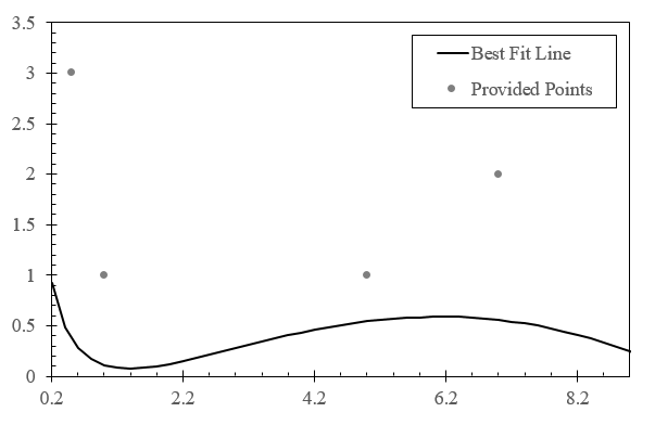
In this example, we will start out with the given points $(. 5, 3)$ , $(1, 1)$ , $(5, 1)$ , $(7, 2)$ . We will fit an equation of the form shown in equation 2.229 to the provided points.

\begin{align} c_{1} x^{2} + c_{2} x + c_{3} \ln (2 x) = y & (2.229) \end{align}

As can be deduced, our task is to find the coefficients $c_{1}$ , $c_{2}$ , and $c_{3}$ . Per laid out process, our problem can be rewritten using equation 2.206 as shown in equation 2.230.

c_{1} [\begin{matrix} . 25 \\ 1 \\ 25 \\ 49 \end{matrix}] + c_{2} [\begin{matrix} . 5 \\ 1 \\ 5 \\ 7 \end{matrix}] + c_{3} [\begin{matrix} 0 \\ - . 69 \\ . 916 \\ 1.25 \end{matrix}] \approx [\begin{matrix} 3 \\ 1 \\ 1 \\ 2 \end{matrix}]

(2.230)

Performing the Gram-Schmidt organization procedure on the vectors provided in equation 2.230 ( ${\vec{a}}_{1}$ , ${\vec{a}}_{2}$ , ${\vec{a}}_{3}$ using previous terminology), we get the following.

{\vec{u}}_{1} = [\begin{matrix} . 25 \\ 1 \\ 25 \\ 49 \end{matrix}]

{\vec{u}}_{2} = [\begin{matrix} . 46 \\ . 84 \\ 1.12 \\ - . 59 \end{matrix}]

{\vec{u}}_{3} = [\begin{matrix} . 046 \\ - . 619 \\ . 356 \\ - . 169 \end{matrix}]

We can find ${\vec{y}}_{f}$ using the equation 2.209 as shown in equation 2.231.

\frac{[\begin{matrix} 3 \\ 1 \\ 1 \\ 2 \end{matrix}] \cdot [\begin{matrix} . 25 \\ 1 \\ 25 \\ 49 \end{matrix}]}{[\begin{matrix} . 25 \\ 1 \\ 25 \\ 49 \end{matrix}] \cdot [\begin{matrix} . 25 \\ 1 \\ 25 \\ 49 \end{matrix}]} [\begin{matrix} . 25 \\ 1 \\ 25 \\ 49 \end{matrix}] + \frac{[\begin{matrix} 3 \\ 1 \\ 1 \\ 2 \end{matrix}] \cdot [\begin{matrix} . 46 \\ . 84 \\ 1.12 \\ - . 59 \end{matrix}]}{[\begin{matrix} . 46 \\ . 84 \\ 1.12 \\ - . 59 \end{matrix}] \cdot [\begin{matrix} . 46 \\ . 84 \\ 1.12 \\ - . 59 \end{matrix}]} [\begin{matrix} . 46 \\ . 84 \\ 1.12 \\ - . 59 \end{matrix}] + \frac{[\begin{matrix} 3 \\ 1 \\ 1 \\ 2 \end{matrix}] \cdot [\begin{matrix} . 046 \\ - . 619 \\ . 356 \\ - . 169 \end{matrix}]}{[\begin{matrix} . 046 \\ - . 619 \\ . 356 \\ - . 169 \end{matrix}] \cdot [\begin{matrix} . 046 \\ - . 619 \\ . 356 \\ - . 169 \end{matrix}]} [\begin{matrix} . 046 \\ - . 619 \\ . 356 \\ - . 169 \end{matrix}] = [\begin{matrix} . 365 \\ 1.291 \\ 1.685 \\ 1.658 \end{matrix}]

(2.231)

Now that we have found ${\vec{y}}_{f}$ , we can assemble the equation laid out by 2.210 as shown in equation 2.232.

c_{1} [\begin{matrix} . 25 \\ 1 \\ 25 \\ 49 \end{matrix}] + c_{2} [\begin{matrix} . 5 \\ 1 \\ 5 \\ 7 \end{matrix}] + c_{3} [\begin{matrix} 0 \\ - . 69 \\ . 916 \\ 1.25 \end{matrix}] = [\begin{matrix} . 365 \\ 1.291 \\ 1.685 \\ 1.658 \end{matrix}]

(2.232)

Solving the systems of equations provided within equation 2.232 for our unknowns, we get $c_{1} = - . 05$ , $c_{2} = . 75$ , and $c_{3} = - . 85$ . Plugging this into our original fitting equation (equation 2.229) we get equation 2.233.

\begin{align} - . 05 x^{2} + . 75 x - . 85 \ln (2 x) = y & (2.233) \end{align}

As laid out previously, we can derive the same solution using matrix techniques. Applying equation 2.221 to this situation, we get equation 2.234 $[A]$ .

[A] = [\begin{matrix} . 25 & . 5 & 0 \\ 1 & 1 & - . 69 \\ 25 & 5 & . 916 \\ 49 & 7 & 1.25 \end{matrix}]

(2.234)

Plugging in equation 2.234 along with the given $\vec{y}$ into equation 2.228 we get equation 2.235.

[\begin{matrix} c_{1} \\ c_{2} \\ c_{3} \end{matrix}] = {({[\begin{matrix} . 25 & . 5 & 0 \\ 1 & 1 & - . 69 \\ 25 & 5 & . 916 \\ 49 & 7 & 1.25 \end{matrix}]}^{T} [\begin{matrix} . 25 & . 5 & 0 \\ 1 & 1 & - . 69 \\ 25 & 5 & . 916 \\ 49 & 7 & 1.25 \end{matrix}])}^{- 1} {[\begin{matrix} . 25 & . 5 & 0 \\ 1 & 1 & - . 69 \\ 25 & 5 & . 916 \\ 49 & 7 & 1.25 \end{matrix}]}^{T} [\begin{matrix} 3 \\ 1 \\ 1 \\ 2 \end{matrix}]

(2.235)

Solving, we end up with equation 2.236.

[\begin{matrix} c_{1} \\ c_{2} \\ c_{3} \end{matrix}] = [\begin{matrix} - . 05 \\ . 752 \\ - . 853 \end{matrix}]

(2.236)

This result matches the result we obtained using the non-matrix method.

In Figure 2.7, a graph of 2.233 is provided along with the points provided in the problem statement.

Figure 2.7: Graph of best fit line (equation 2.233) as compared to the points provided in the problem statement

2.4.1 R Squared

The $R^{2}$ statistic is a tool to determine how closely our best fit function fits to the given data-set. This statistic is calculated using equation 2.237.

\begin{align} R^{2} = 1 - \frac{\sum {(y_{i} - ȳ)}^{2}}{\sum {(y_{i} - f (x_{i}))}^{2}} & (2.237) \end{align}

In equation 2.237, $ȳ$ is the mean given $y$ value. $f (x)$ corresponds to the best fit function whose generation has been detailed in section 2.4.

As can be deduced from equation 2.237, an $R^{2}$ of $1$ means that the best fit function perfectly models the data (goes through all the points). The closer the $R^{2}$ statistic is to $0$ , the worse of a fit exists.

Short Example

In this example, we will generate an $R^{2}$ static for the example provided in section 2.4. As a reminder, we were provided the following data-set; $(. 5, 3)$ , $(1, 1)$ , $(5, 1)$ , $(7, 2)$ . We used this data-set to generate the following best fit equation.

\begin{array}{l} - . 05 x^{2} + . 752 x - . 853 \ln (2 x) = f (x) \end{array}

We can use this data to generate Table 2.3.

Table 2.3: Table showing

x

y

(provided value),

ȳ

(mean), and

f (x)

(estimate from the best fit equation).

$x$	$y$	$ȳ$	$f (x)$

$. 5$	$3$	$1.75$	$. 36$
$1$	$1$	$1.75$	$. 11$
$5$	$1$	$1.75$	$. 55$
$7$	$2$	$1.75$	$. 56$

Plugging this data into equation 2.237 we get an $R^{2}$ value of $- 2.64$ . The fact that this value is negative signifies that the data-set has a greater variation from the best fit function than from it’s own mean.