Calculus Fundamentals

2.1 Calculus Fundamentals

Calculus is defined as the branch of mathematics that utilizes infinitesimally small quantities to study continuous change. The two main topics within calculus are the derivative and the integral.

2.1.1 The Derivative

In order to understand the derivative, we will start with a two variables ( $x, y$ ). These variables are related to each other by the function presented in equation 2.1.

\begin{align} y = f (x) & (2.1) \end{align}

Our goal is to find how much $y$ varies per increment of $x$ . This ”quantity of change per unit $x$ ” is symbolized by the variable $C$ . In order to do this, we can start out with equation 2.2.

\begin{align} C = \frac{y_{2} - y_{1}}{x_{2} - x_{1}} & (2.2) \end{align}

Equation 2.2 will tell us how much $y$ changes from $x_{1}$ to $x_{2}$ . However, we are interested in the amount $y$ is changed instantaneously. Therefore, we can say that $x_{2} = x_{1} + h$ where $h$ is an infinitesimally small quantity. Plugging this into equation 2.2 we get equation 2.3.

\begin{align} C = \lim_{h \to 0} \frac{y_{2} - y_{1}}{(x_{1} + h) - x_{1}} & (2.3) \end{align}

Simplifying the denominator of equation 2.3 and plugging in equation 2.1 we get equation 2.4.

\begin{align} C = \lim_{h \to 0} \frac{f (x + h) - f (x)}{h} & (2.4) \end{align}

Please note that since we are now dealing with one value of $x$ , we replaced $x_{1}$ with $x$ . The above equation can be used to find the instantaneous change in $y$ per infinitesimally small interval $x$ for any value $x$ . Typically, we replace $C$ with the following notation.

\begin{align} \frac{𝑑𝑦}{𝑑𝑥} = \lim_{h \to 0} \frac{f (x + h) - f (x)}{h} & (2.5) \end{align}

The $\frac{𝑑𝑦}{𝑑𝑥}$ symbolizes ”The change in $y$ per a infinitesimally small interval $x$ ”.

Short Example

Let us start with the function shown in equation 2.6.

\begin{align} p = t^{2} & (2.6) \end{align}

For the purpose of this example, let us assume that $p$ is the position of a particle at any time $t$ . We want to find the instantaneous change in $p$ per interval $t$ . You may notice that this is position divided by time ... we are calculating speed. Plugging equation 2.6 into equation 2.5 we get equation 2.7.

\begin{align} \frac{𝑑𝑝}{𝑑𝑡} = \lim_{h \to 0} \frac{{(t + h)}^{2} - t^{2}}{h} & (2.7) \end{align}

Solving the limit in equation 2.7, we get equation 2.8.

\begin{align} \frac{𝑑𝑝}{𝑑𝑡} = 2 t & (2.8) \end{align}

The Chain Rule

Finding the limit of complicated functions using equation 2.5 is very difficult. Therefore, calculus students typically memorize series of rules which correspond to the derivatives of functions. One of the most fundamental derivation rules is the chain rule. The chain rule deals with derivatives of functions within functions. Consider the function provided in equation 2.9.

\begin{align} f (x) = h (g (x)) & (2.9) \end{align}

To simply equation 2.9, we can state $y = g (x)$ . The chain rule then states $𝑑𝑓 ∕ 𝑑𝑥$ can be found using equation 2.10.

\begin{align} \frac{𝑑𝑓}{𝑑𝑥} = \frac{𝑑h (y)}{𝑑𝑦} \frac{𝑑𝑔 (x)}{𝑑𝑥} & (2.10) \end{align}

Essentially, you take the derivative of the outside function first, treating the inside function as a variable, and then take the derivative of the inside function.

The Product Rule

Consider a function $f (x)$ which consists of the product of two separate functions $g (x)$ and $h (x)$ , as shown in equation 2.11.

\begin{align} f (x) = g (x) * h (x) & (2.11) \end{align}

The product rule states that the derivative of $f (x)$ can be calculated using equation 2.12.

\begin{align} \frac{𝑑𝑓}{𝑑𝑥} = \frac{𝑑𝑔}{𝑑𝑥} * h (x) + g (x) * \frac{𝑑h}{𝑑𝑥} & (2.12) \end{align}

The product rule can be derived by use of equation 2.5. However, calculus proofs are outside of the scope of this book.

The Quotient Rule

Consider a function $f (x)$ which consists of the quotient of two separate functions $g (x)$ and $h (x)$ , as shown in equation 2.13.

\begin{align} f (x) = \frac{g (x)}{h (x)} & (2.13) \end{align}

The quotient rule states that the derivative of $f (x)$ is as shown in equation 2.14.

\begin{align} \frac{𝑑𝑓}{𝑑𝑥} = \frac{\frac{𝑑𝑔}{𝑑𝑥} * h (x) - g (x) * \frac{𝑑h}{𝑑𝑥}}{{(h (x))}^{2}} & (2.14) \end{align}

The quotient rule can be derived by use of equation 2.5. However, calculus proofs are outside of the scope of this book.

2.1.2 The Partial Derivative

The partial derivative is used when we differentiate a function with more than two variables. An example of such a function is shown in equation 2.15.

\begin{align} z = f (x, y) & (2.15) \end{align}

Now, we need to make a decision. Are we interested in finding out how much $z$ changes per increment of $y$ ? Or are we interested in finding out how much $z$ changes per increment of $x$ ? Lets go with the change of $z$ with respect to $x$ . This change can be expressed using equation 2.16.

\begin{align} C = \frac{z_{2} - z_{1}}{x_{2} - x_{1}} & (2.16) \end{align}

Following the example from section 2.1.1, equation 2.16 will tell us how much $z$ changes from $x_{1}$ to $x_{2}$ . However, we are interested in the amount $z$ is changed instantaneously. Therefore, we can say that $x_{2} = x_{1} + h$ where $h$ is an infinitesimally small quantity. Plugging this into equation 2.16 we get equation 2.17.

\begin{align} \frac{∂𝑧}{∂𝑥} = \lim_{h \to 0} \frac{f (x + h, y) - f (x, y)}{h} & (2.17) \end{align}

Please note that in equation 2.17, the denominator was simplified and equation 2.15 was plugged in. The $∂𝑧 ∕ ∂𝑥$ notation mimics the $𝑑𝑦 ∕ 𝑑𝑥$ notation from equation 2.5. However, the fancy $\partial$ emphasizes that this is a partial derivative. Partial referrers to the fact that we are finding the change in $z$ with respect to one out of two possible variables. We can repeat the proceeding process to find $∂𝑧 ∕ ∂𝑦$ .

Short Example

Let us start with the function in equation 2.18.

\begin{align} z = x^{2} + y^{2} + 𝑥𝑦 & (2.18) \end{align}

We are interested in finding $∂𝑧 ∕ ∂𝑥$ . In order to do this, we use equation 2.17 accordingly.

\begin{array}{l} \frac{∂𝑧}{∂𝑥} = \lim_{h \to 0} \frac{[{(x + h)}^{2} + (x + h) y + y^{2}] - [x^{2} + 𝑥𝑦 + y^{2}]}{h} \end{array}

Solving the limit, we are left with equation 2.19.

\begin{align} \frac{∂𝑧}{∂𝑥} = 2 x + y & (2.19) \end{align}

In order to provide a visualization, a graph of the function in equation 2.18 with the $y = 0$ plane overlaid is provided in Figure 2.1. The derivative of the grey line is $\frac{∂𝑧}{∂𝑥}$ at $y = 0$ .

Figure 2.1: Graph of equation 2.18 with the $y = 0$ plane overlaid. The derivative of the grey line is $\frac{∂𝑧}{∂𝑥}$ at $y = 0$ .

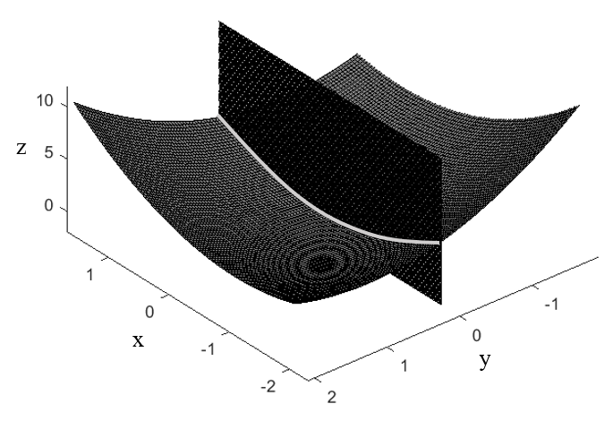
The partial derivative simply constrains the original function $z$ to a two dimensional plane and then finds the derivative (section 2.1.1) on that plane.

2.1.3 The Integral

In the derivative sections, we reviewed a method for finding the change in a variable (in section 2.1.1 this was $y$ ) per an interval of another variable (in section 2.1.1 this was $x$ ). This process can also be thought of as a type of instantaneous division. We divide the change in $y$ by the change in $x$ , given that the change in $x$ is infinitesimally small. The integral can be thought of as the opposite of the derivative; instead of dealing with instantaneous division, it deals with instantaneous multiplication.

To understand the integral, let us begin with the function shown in equation 2.20.

\begin{align} y = f (x) & (2.20) \end{align}

Our goal is to multiply $y$ by some interval $Δ x_{𝑡𝑜𝑡}$ . $Δ x_{𝑡𝑜𝑡}$ is equal to $x_{B} - x_{A}$ . The result of the multiplication will be represented by $M$ . Since $y$ varies as a function of $x$ , we need to use the the series shown in equation 2.21 for such a multiplication.

\begin{align} M = f (x_{1}) * Δ x_{1 \to 2} + f (x_{2}) * Δ x_{2 \to 3} + f (x_{3}) * Δ x_{3 \to 4} + . . . & (2.21) \end{align}

Essentially, we are freezing the continuous $f (x)$ function at points $x_{1}$ , $x_{2}$ , $x_{3}$ (and so forth) and then multiplying this function by an incremental $Δ x$ , which is the distance between each frozen $x$ value. Naturally, $Δ x_{1 \to 2} + Δ x_{2 \to 3} + Δ x_{3 \to 4} + . . .$ must equal the total interval $Δ x_{𝑡𝑜𝑡}$ ( $x_{B} - x_{A}$ ).

We also set up the above sequence so that each incremental $Δ x$ value is of the same quantity. Therefore, $Δ x_{1 \to 2} = Δ x_{2 \to 3} = Δ x_{3 \to 4} = . . . = Δ x_{𝑖𝑛𝑐}$ . The $Δ x_{𝑖𝑛𝑐}$ stands for $x$ incremental and will be used from now on. If we want to find the value of $Δ x_{𝑖𝑛𝑐}$ we can use equation 2.22.

\begin{align} Δ x_{𝑖𝑛𝑐} = \frac{x_{B} - x_{A}}{n} & (2.22) \end{align}

In equation 2.22 $n$ is the total amount of terms we use to calculate $M$ . Plugging in equation 2.22 into equation 2.21 we get equation 2.23.

\begin{aligned} M = f (\frac{x_{B} - x_{A}}{n}) Δ x_{𝑖𝑛𝑐} + f (\frac{x_{B} - x_{A}}{n} + \frac{x_{B} - x_{A}}{n}) Δ x_{𝑖𝑛𝑐} + \\ f (\frac{x_{B} - x_{A}}{n} + \frac{x_{B} - x_{A}}{n} + \frac{x_{B} - x_{A}}{n}) Δ x_{𝑖𝑛𝑐} + . . . \end{aligned}

(2.23)

We can rewrite equation 2.23 as a series as shown in equation 2.24.

M = \sum_{i = 1}^{n} f (\frac{x_{B} - x_{A}}{n} * i) * \frac{x_{B} - x_{A}}{n}

(2.24)

How, here is the fun part. The more $n$ terms we have, the more ”accurate” our result will become because we will be freezing $f (x)$ at more locations. Therefore, ideally, $n = \infty$ . We can rewrite equation 2.24 to include a limit for $n$ approaching infinity. This is shown in equation 2.25.

\int_{x_{A}}^{x_{B}} f (x) 𝑑𝑥 = \lim_{n \to \infty} \sum_{i = 1}^{n} f (\frac{Δ x_{𝑡𝑜𝑡}}{n} * i) * \frac{Δ x_{𝑡𝑜𝑡}}{n}

(2.25)

In equation 2.25, $M$ was replaced by the $\int_{x_{A}}^{x_{B}} f (x) 𝑑𝑥$ . The $\int$ is called the integral sign and represents a big elongated S, which stands for sum. The integral is, as shown in the above sequences, a repeated sum. As stated previously, $x_{A}$ and $x_{B}$ are the lower and upper bounds of $Δ x$ . $𝑑𝑥$ represents $Δ x_{𝑖𝑛𝑐}$ which is multiplied and added an infinite amount of times, with the goal of multiplying $f (x)$ by $Δ x_{𝑡𝑜𝑡}$ .

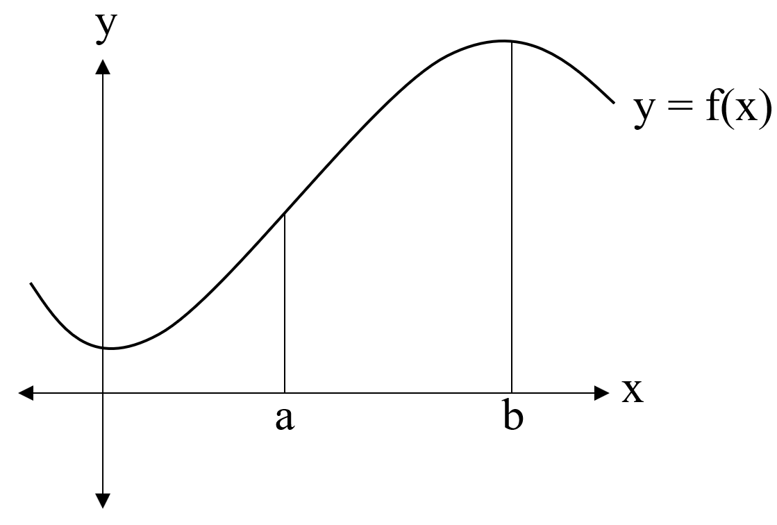
The integral can be easily visualized as the area under a curve, as shown in Figure 2.2.

Figure 2.2: Visualization of $\int_{a}^{b} f (x) 𝑑𝑥$ . The value of the integral is the area of the region bounded by $f (x)$ from the top, the $x$ axis from the bottom, $a$ on the left, and $b$ on the right.

A short example

Let us begin with the function in equation 2.26.

v = 2 t

(2.26)

We are interested in integrating (multiplying) this term by the interval $0 \to t_{f}$ . For the purpose of this example, let us assume that $v$ is velocity and $t$ is time. You may notice that we are multiplying velocity by an interval of time ( $0 \to t_{f}$ )... we are calculating position traveled during the time period $0 \to t_{f}$ . Plugging in equation 2.26 to equation 2.25 we get equation 2.27.

\int_{0}^{t_{f}} 2 𝑡𝑑𝑡 = \lim_{n \to \infty} \sum_{i = 1}^{n} 2 (\frac{t_{f}}{n} * i) * \frac{t_{f}}{n}

(2.27)

Simplifying equation 2.27, we get equation 2.28.

\int_{0}^{t_{f}} 2 𝑡𝑑𝑡 = \lim_{n \to \infty} \sum_{i = 1}^{n} 2 {(\frac{t_{f}}{n})}^{2} * i

(2.28)

Part of this sequence actually has a known solution shown in equation 2.29.

\sum_{n = 1}^{n} i = \frac{n (n + 1)}{2}

(2.29)

There are numerous visual and traditional mathematical proofs for the series sum shown in equation 2.29. These will not be covered in this book. Since we know that $\frac{t_{f}}{n}$ is a constant, we can plug in equation 2.29 into equation 2.28 to get equation 2.30.

\int_{0}^{t} 2 𝑡𝑑𝑡 = \lim_{n \to \infty} 2 {(\frac{t_{f}}{n})}^{2} * \frac{n (n + 1)}{2}

(2.30)

Evaluating the limit in equation 2.30, we get equation 2.31.

\int_{0}^{t} 2 𝑡𝑑𝑡 = t_{f}^{2}

(2.31)

You may notice that this gave us the exact same output as equation 2.6. We essentially just undid what was done in the example in section 2.1.1.0. This solidifies the concept that the integral is the opposite of a derivative.

2.1.4 Double (and beyond) Integrals

In section 2.1.3 we reviewed how to multiply $y$ by an interval $Δ x_{𝑡𝑜𝑡}$ if $y$ varies as a function of $x$ . In this section, we expand the definition of the integral to make it compatible with multiple variables. In order to do this, let us begin with equation 2.32.

\begin{align} z = f (x, y) & (2.32) \end{align}

Our goal is to multiply $z$ by some interval $Δ x_{𝑡𝑜𝑡}$ and $Δ y_{𝑡𝑜𝑡}$ . $Δ x_{𝑡𝑜𝑡}$ is equal to $x_{B} - x_{A}$ . $Δ y_{𝑡𝑜𝑡}$ is equal to $y_{B} - y_{A}$ . Plugging this into equation 2.25 we get equation 2.33.

\int_{y_{A}}^{y_{B}} \int_{x_{A}}^{x_{B}} f (x, y) 𝑑𝑥𝑑𝑦 = \lim_{n \to \infty} \sum_{j = 1}^{n} \sum_{i = 1}^{n} f (\frac{Δ x_{𝑡𝑜𝑡}}{n} * i, \frac{Δ y_{𝑡𝑜𝑡}}{n} * j) * \frac{Δ x_{𝑡𝑜𝑡}}{n} * \frac{Δ y_{𝑡𝑜𝑡}}{n}

(2.33)

As with the single integral, we are finding $z$ at each incremental location $x, y$ and multiplying this value by the interval $Δ x_{𝑖𝑛𝑐}$ and $Δ y_{𝑖𝑛𝑐}$ . All these “multiplications” are then added together. In equation 2.33, we first iterate through all $x$ intervals with $j$ fixed at 1, and then move on to $j = 2$ and so forth. This makes $x$ the inner integration variable and $y$ the outer integration variable. However, since this is all multiplication and addition it does not matter which order we use. The solution to $\int \int f (x, y) 𝑑𝑥𝑑𝑥$ is the same as $\int \int f (x, y) 𝑑𝑦𝑑𝑥$ .

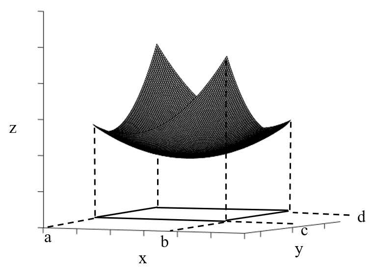
The double integral can be easily visualized as the volume under a surface, as shown in Figure 2.3.

Figure 2.3: Visualization of $\int_{c}^{d} \int_{a}^{b} f (x, y) 𝑑𝑥𝑑𝑦$ . The value of the integral is the volume of the region bounded by $f (x, y)$ from the top and the $x - y$ plane from the bottom within the bounds of $x = a$ to $x = b$ and $y = c$ to $y = d$ .

We can follow a similar pattern for variables that are a function of three (or more) variables. In this case we would get a triple (or more) integral.

A short example

Let us begin with the function provided in equation 2.34.

z = 𝑥𝑦

(2.34)

We are interested in integrating (multiplying) this term by the interval $0 \to x_{f}$ and $0 \to y_{f}$ . Plugging the equation 2.34 into equation 2.33 we get equation 2.35.

\int_{0}^{y_{f}} \int_{0}^{x_{f}} f (x, y) 𝑑𝑥𝑑𝑦 = \lim_{n \to \infty} \sum_{j = 1}^{n} \sum_{i = 1}^{n} (\frac{x_{f}}{n} * i) (\frac{y_{f}}{n} * j) * \frac{x_{f}}{n} * \frac{y_{f}}{n}

(2.35)

As before, part of this sequence actually has a known solution shown in equation 2.36.

\sum_{n = 1}^{n} i = \frac{n (n + 1)}{2}

(2.36)

Plugging equation 2.36 into equation 2.35 and simplifying we get equation 2.37.

\int_{0}^{y_{f}} \int_{0}^{x_{f}} f (x, y) 𝑑𝑥𝑑𝑦 = \lim_{n \to \infty} \frac{x_{f}^{2} y_{f}^{2}}{n^{4}} \frac{n (n + 1)}{2} \sum_{j = 1}^{n} j

(2.37)

Now we can plug in equation 2.36 again; given that we replace $i$ with $j$ . Doing this we, are left with the limit provided in equation 2.38.

\int_{0}^{y_{f}} \int_{0}^{x_{f}} f (x, y) 𝑑𝑥𝑑𝑦 = \lim_{n \to \infty} \frac{x_{f}^{2} y_{f}^{2}}{n^{4}} \frac{n (n + 1)}{2} \frac{n (n + 1)}{2}

(2.38)

Evaluating the limit in equation 2.38, we obtain the answer as shown in equation 2.39.

\int_{0}^{y_{f}} \int_{0}^{x_{f}} f (x, y) 𝑑𝑥𝑑𝑦 = \frac{1}{4} x_{f}^{2} y_{f}^{2}

(2.39)

2.1.5 Methods of Integration

The integral is defined in equation 2.25. Considering we are dealing with an sum with a number of terms which approach infinity, finding a solution for any function can be very hard. In the short examples provided for both the integral and double integral we used the convenient identity $\sum_{n = 1}^{n} i = \frac{n (n + 1)}{2}$ . However, not every function has a closed form equation for a given sum. In practice, integrals are usually solved with the help of known base function integrals. Algebraic manipulations are used to simplify an original function into one in the form of such base functions, allowing for easier integration. In this section, three common algebraic manipulations used to simplify integrals are provided. This is not a comprehensive list; there are other methods such as trig substitution which are also used to simplify integrals. However, the methods included in this section are deemed most relevant.

U Substitution

U substitution is a process of reversing the chain rule (the chain rule is introduced in section 2.1.1.0). Consider the integral shown in equation 2.40.

\int \frac{𝑑𝑓 (g (x))}{𝑑𝑥} \frac{𝑑𝑔 (x)}{𝑑𝑥} 𝑑𝑥

(2.40)

By using the substitution $u = g (x)$ we can rewrite the equation 2.40 as shown in equation 2.41.

\int \frac{𝑑𝑓 (u)}{𝑑𝑥} 𝑑𝑢

(2.41)

The idea here is equation 2.41 is simpler to look at and therefore easier for to integrate.

Short Example

Consider the function provided in equation 2.42.

\int_{0}^{x} 2 x \cos (x^{2}) 𝑑𝑥

(2.42)

Setting $u = x^{2}$ , we can rewrite the equation 2.42 as shown in equation 2.43.

\int_{0}^{x} \cos (u) 𝑑𝑢

(2.43)

It is given that $\int \cos (u) = \sin (u)$ . Therefore, plugging $u$ back in, our final answer is obtained as shown in equation 2.44.

\int_{0}^{x} 2 x \cos (x^{2}) 𝑑𝑥 = \sin (x^{2})

(2.44)

Integration by Parts

Integration by Parts is a way of reducing the power of a term within a two term integral. The integration by parts identity is provided in equation 2.45.

\int f (x) d (g (x)) = f (x) g (x) - \int g (x) d (f (x))

(2.45)

Short Example

Consider the function provided in equation 2.46.

\int_{0}^{x} x \cos (x) 𝑑𝑥

(2.46)

Let us define the above equation in terms of equation 2.45. $f (x) = x$ , and $\frac{𝑑𝑔 (x)}{𝑑𝑥} = \cos (x)$ . Therefore, $g (x) = \sin (x)$ . Plugging this all into equation 2.45 we are left with equation 2.47.

\int_{0}^{x} x \cos (x) 𝑑𝑥 = x \sin (x) - \int \sin (x) 𝑑𝑥

(2.47)

The integral in equation 2.47 simplifies so nicely because $\frac{d (f (x))}{𝑑𝑥} = 1$ .

Partial Fraction Decomposition

From algebra, we know the identity provided in equation 2.48 is true.

\frac{C_{1}}{g (x)} + \frac{C_{2}}{f (x)} = \frac{𝐴𝑓 (x) + 𝐵𝑔 (x)}{f (x) g (x)}

(2.48)

Equation 2.48, $C_{1}$ and $C_{2}$ are both known constants. The partial fraction decomposition technique is a method of doing the opposite of this operation. Essentially, given $\frac{C_{1} f (x) + C_{2} g (x)}{f (x) g (x)}$ we want to get $\frac{C_{1}}{g (x)} + \frac{C_{2}}{f (x)}$ . The reason we want to decompose polynomial fractions in this way is because it is easier to integrate $\frac{C_{1}}{g (x)} + \frac{C_{2}}{f (x)}$ than it is to integrate $\frac{C_{1} f (x) + C_{2} g (x)}{f (x) g (x)}$ .

The first step in a fraction decomposition is to write an equation in the general format provided in equation 2.49.

\frac{C_{1} f (x) + C_{2} g (x)}{f (x) g (x)} = \frac{A}{g (x)} + \frac{B}{f (x)}

(2.49)

In equation 2.49, $A$ and $B$ are both unknown constants. Multiplying both sides of equation 2.49 by $\frac{f (x) g (x)}{f (x) g (x)}$ we get equation 2.50.

C_{1} f (x) + C_{2} g (x) = 𝐴𝑓 (x) + 𝐵𝑔 (x)

(2.50)

From here it is quite obvious that $A = C_{1}$ and $B = C_{2}$ . In the case of more complicated algebra, a system of equations can be used to find $A$ and $B$ .

There are some specific rules regarding situations where the denominator of the original equation is at a given power (for example ${[f (x)]}^{k}$ ) or when the power of the denominator is greater than 1 (for example $a x^{2} + 𝑏𝑥 + c$ ). The goal here is to provide a method overview and therefore we will not go over how to do partial fraction decomposition in these specific cases.

Short Example

Suppose we tasked with solving the integral in equation 2.51.

\int \frac{5 x - 4}{x^{2} - x - 2} 𝑑𝑥

(2.51)

Factoring the denominator of equation 2.51 and using equation 2.49 we get the equation 2.52.

\frac{5 x - 4}{(x + 1) (x - 2)} = \frac{A}{x - 2} + \frac{B}{x + 1} =

(2.52)

Multiplying equation 2.52 by $(x + 1) (x - 2)$ we get equation 2.53.

5 x - 4 = A (x + 1) + B (x - 2)

(2.53)

Now, we can plug in 2 different values for $x$ . It doesn’t matter which values. We will be then left with 2 equations and two unknowns. Solving this system of equations, we get $A = 2$ and $B = 3$ . We can plug these values into equation 2.52, and then plug this new identity into the original integral. Doing this, we are left with equation 2.54.

\int \frac{2}{x - 2} + \frac{3}{x + 1} 𝑑𝑥

(2.54)

The integral in equation 2.54 is easier to integrate than the integral in equation 2.51, although they are equivalent.